Population Ecology

1. Population Ecology

2. Population Ecology • Populations in Space and Time • Types of Ecological Interactions • Fluctuations in Population Densities • Population Fluctuations • Variations in Species’ Ranges • Managing Populations • Regional and Global Processes Influence Local Population Dynamics

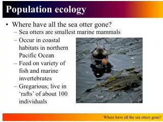
3. Populations in Space and Time • The individuals of a species with a given area constitute a population. • The distribution of the ages of individuals in a population and the way those individuals are distributed over the environment describe the population structure. • Ecologists study population structure at different spatial scales, ranging from local subpopulations to entire species. • The number of individuals of a species per unit of area (or volume) is its population density.

4. Populations in Space and Time • Ecologists are interested in population densities because dense populations often exert strong influences on their own members as well as on populations of other species. • Density of terrestrial organisms is measured as number of individuals per unit area. • Density of aquatic organisms is measured as individuals per unit volume. • For some species such as plants, the biomass or percentage of ground covered may be a more useful measure of density than the number of individuals.

5. Populations in Space and Time • The structure of a population changes continually because of demographic events—births, deaths, immigration, and emigration. • Population dynamics is the change in population density through time and space. • Demography is the study of birth, death, and movement rates that give rise to population dynamics.

6. Populations in Space and Time • Population dynamics can be represented by: • N1 = N0 + B – D + I – E • N1 = number of individuals at time 1 • N0 = number of individuals at time 0 • B = number of individuals born between time 0 and time 1 • D = number of individuals that died between time 0 and time 1 • I = number of individuals that immigrated • E = number of individuals that emigrated

7. Populations in Space and Time • Life table information can be used to predict future trends in populations. • A cohort is a group of individuals that were born at the same time. • A life table can be constructed by determining the number of individuals in a cohort that are still alive at specific times (the survivorship) and the number of offspring they produced in each time interval.

8. Table 54.1 Life Table of the 1978 Cohort of the Cactus Finch on Isla Daphne (Part 1)

9. Table 54.1 Life Table of the 1978 Cohort of the Cactus Finch on Isla Daphne (Part 2)

10. Populations in Space and Time • The life table for a cohort of the cactus finch on Isla Daphne in the Galápagos archipelago shows that mortality rates were initially high, leveled off, and again increased as the birds aged. • Mortality rate also fluctuated through the years because survival depends upon seed production, and seed production is correlated with rainfall.

11. Populations in Space and Time • Survivorship curves in many populations fall into one of three patterns. • In some populations (e.g., humans in the U.S.), most individuals survive for most of their potential life span and die at about the same age. • In some (e.g., songbirds), the probability of surviving over the life span is the same once individuals are a few months old. • In species that produce a large number of offspring and provide little parental care, high death rates for the young are followed by high survival rates during the middle of the life span.

12. Figure 54.1 Survivorship Curves (Part 1)

13. Figure 54.1 Survivorship Curves (Part 2)

14. Populations in Space and Time • The age distribution of individuals in a population reveals much about the recent history of births and deaths. • For example, in the U.S., population size increased during the “baby boom” of the 1950s and again during the “baby boom echo” of the 1980s. • Life tables can help us to understand why population densities change over time and to determine which groups should be the focus of efforts to save rare species.

15. Figure 54.2 Age Distributions Change over Time

16. Types of Ecological Interactions • Species interactions fall into several categories. • If both participants benefit from an interaction, the interaction is a mutualism (+/+ interaction). • An example of mutualism is the association between plants and soil fungi called mycorrhizae, or between plants and nitrogen-fixing bacteria. • Corals gain most of their energy from photosynthetic protists. The protists get nutrients when the corals digest animals. • Termites have protists in their gut that digest cellulose; they provide the protists, in turn, with nutrients.

17. Types of Ecological Interactions • If one participant benefits but the other is unaffected, the interaction is a commensalism (+/0 interaction). • Cattle egrets forage for insects near large mammals, and the movements of the large animal flush out insects, which the birds eat. The mammal does not gain or lose anything from this interaction.

18. Figure 54.3 Commensalism Benefits One Partner

19. Types of Ecological Interactions • If one participant is harmed but the other is unaffected, the interaction is an amensalism (0/– interaction). • Trees and branches falling from trees damage smaller plants beneath them; this is an example of amensalism.

20. Types of Ecological Interactions • One organism may benefit itself while harming another organism; these interactions are called predator–prey and parasite–host interactions (+/– interactions). • If two organisms use the same resources and those resources are insufficient for their combined needs, they are in competition (–/– interaction).

21. Table 54.2 Types of Ecological Interactions

22. Factors Influencing Population Densities • Species that use abundant resources often reach higher population densities than species that use scarce resources. • Species with small individuals generally reach higher population densities than species with large individuals. • This relationship can be demonstrated by a logarithmic plot of population density against body size for a variety of mammals worldwide.

23. Figure 54.4 Population Density Decreases as Body Size Increases

24. Factors Influencing Population Densities • Newly introduced species often reach high population densities. • An example is species introduced into a region where their normal predators and diseases are absent. • Zebra mussels whose larvae were carried from Europe in the ballast water of ships now occupy much of the Great Lakes and Mississippi River drainage. • Complex social organizations (e.g., ants, termites, humans) may facilitate high densities.

25. Figure 54.5 Introduced Zebra Mussels Have Spread Rapidly

26. Fluctuations in Population Densities • If a single bacterium were allowed to grow and reproduce in an unlimited environment, explosive population growth would result. • Within a month, the bacterial colony would weigh as much as the visible universe and would be expanding outward at the speed of light. • But while populations do fluctuate in density, even the most dramatic fluctuations are less than what is theoretically possible.

27. Fluctuations in Population Densities • All populations have the potential for explosive growth because, as the number of individuals in the population increases, the number of new individuals added per unit of time accelerates, even if the rate per capita of population increase remains constant. • If births and deaths occur continuously and at constant rates, a graph of the population size over time forms a J-shaped curve that describes a form of explosive growth called exponential growth.

28. Figure 54.6 Exponential Population Growth (Part 1)

29. Figure 54.6 Exponential Population Growth (Part 2)

30. Fluctuations in Population Densities • Exponential growth can be represented mathematically: DN/Dt = (b – d)N • DN = the change in number of individuals • Dt = the change in time • b = the average per capita birth rate (includes immigrations) • d = the average per capita death rate (includes emigrations)

31. Fluctuations in Population Densities • The difference between per capita birth rate (b) and per capita death rate (d) is the net reproductive rate (r). • When conditions are optimal, r is at its highest value (rmax), called the intrinsic rate of increase. • rmax is characteristic for a species. • The equation for population growth can be written D/Dt = rmaxN

32. Fluctuations in Population Densities • For limited time periods, some populations may grow at rates close to rmax. • Real populations do not grow exponentially for long because of environmental limitations. • Environmental limitations include food, nest sites, shelter, disease, and predation. • The carrying capacity of an environment (K) is the maximum number of individuals of a species it can support. • Natural population growth more closely resembles an S-shaped curve.

33. Figure 54.7 Logistic Population Growth

34. Fluctuations in Population Densities • The mathematical representation of this type of growth (logistic growth) is: DN/Dt = r[(K – N)/K]N • The equation for logistic growth indicates that the population’s growth slows as it approaches its carrying capacity (K). • Population growth stops when N = K.

35. Fluctuations in Population Densities • Per capita birth and death rates usually fluctuate in response to population density; that is, they are density-dependent. • As a population increases in size, it may deplete its food supply, reducing the amount of food each individual gets. Poor nutrition may increase death rates and decrease birth rates. • If predators are able to capture a larger proportion of the prey when prey density increases, the per capita death rate of the prey rises. • Diseases, which may increase death rates, spread more easily in dense populations than in sparse populations.

36. Fluctuations in Population Densities • Factors that affect birth and death rates in a population independent of its density are said to be density-independent. • For example, a severely cold winter may kill large numbers of a population regardless of its density.

37. Fluctuations in Population Densities • Fluctuations in population density are determined by all the factors acting on it. • In a population of song sparrows, death rates are high during very cold winters regardless of population density (density-independent). • However, the larger the number of breeding males (density-dependent), the larger the number that fail to gain territories and have little chance of reproducing. • The larger the number of breeding females, the fewer offspring each female fledges. The more birds alive in the autumn, the poorer are the chances that juveniles born that year will survive the winter.

38. Figure 54.8 Regulation of an Island Population of Song Sparrows (Part 1)

39. Figure 54.8 Regulation of an Island Population of Song Sparrows (Part 2)

40. Population Fluctuations • A comparison between the cactus finch and the south polar skua shows that some populations fluctuate widely and others fluctuate remarkably little. • Species with long-lived individuals that have low reproductive rates typically have more stable populations than species with short-lived individuals and high reproductive rates. • Small, short-lived individuals generally are more vulnerable to environmental changes.

41. Figure 54.9 Population Sizes May Be Stable or Highly Variable

42. Population Fluctuations • Episodic reproduction can generate fluctuations. • In Lake Erie, 1944 was such an excellent year for reproduction of whitefish that they dominated catches in the lake for several years. • Most of the black cherry trees in a Wisconsin forest in 1971 had become established between 30 and 40 years earlier.

43. Figure 54.10 Individuals Born During Years of Good Reproduction May Dominate Populations (1)

44. Figure 54.10 Individuals Born During Years of Good Reproduction May Dominate Populations (2)

45. Population Fluctuations • Densities of populations that depend on limited resources fluctuate more than those that use a greater variety of resources. • The cactus finch populations fluctuate with the annual production of seeds that they eat. • Many northern coniferous trees reproduce synchronously and episodically. There are years of massive production and years with little seed production. Populations of birds and mammals that depend on the seeds fluctuate also.

46. Population Fluctuations • Predator–prey interactions generate fluctuations because predator population growth lags behind growth in prey and the two populations oscillate. • When prey is scarce, its predator is scarce. • When prey becomes plentiful again, the predator population will increase in a staggered fashion.

47. Population Fluctuations • Changes in population density among small mammals and their predators living at high latitudes are the best-known examples of predator–prey interactions. • Experiments with Canada lynx and snowshoe hares revealed that the oscillating cycle of their populations was driven by both predation and food supply for the hares.

48. Figure 54.11 Hare and Lynx Populations Cycle in Nature (Part 1)

49. Figure 54.11 Hare and Lynx Populations Cycle in Nature (Part 2)

50. Figure 54.12 Prey Population Cycles May Have Multiple Causes (Part 1)