Download
1 / 22
230 likes | 562 Views
MATLAB Lecture #3 EGR 271 – Circuit Theory I. Operation. Arithmetic Operation. MATLAB Dot Operation. Addition. +. +. Subtraction. -. -. Multiplication. *. .*. Division. /. ./. Exponentiation. ^. .^. Tables and Graphs in MATLAB

E N D
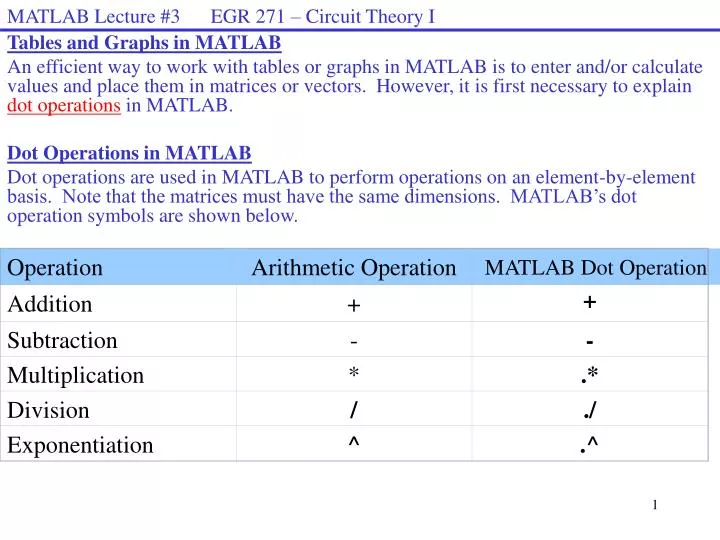
MATLAB Lecture #3 EGR 271 – Circuit Theory I Operation Arithmetic Operation MATLAB Dot Operation Addition + + Subtraction - - Multiplication * .* Division / ./ Exponentiation ^ .^ Tables and Graphs in MATLAB An efficient way to work with tables or graphs in MATLAB is to enter and/or calculate values and place them in matrices or vectors. However, it is first necessary to explain dot operationsin MATLAB. Dot Operations in MATLAB Dot operations are used in MATLAB to perform operations on an element-by-element basis. Note that the matrices must have the same dimensions. MATLAB’s dot operation symbols are shown below.
MATLAB Lecture #3 EGR 271 – Circuit Theory I Dot Operations in MATLAB If matrices A and B have the same dimensions, dot operations work as follows: C = A + B implies that C(i,j) = A(i,j) + B(i,j) D = A - B implies that D(i,j) = A(i,j) - B(i,j) E = A .* B implies that E(i,j) = A(i,j) * B(i,j) F = A ./ B implies that F(i,j) = A(i,j) / B(i,j) G = A .^ B implies that D(i,j) = A(i,j) ^ B(i,j) Example MATLAB program: Results
MATLAB Lecture #3 EGR 271 – Circuit Theory I Generating a Range of Values in MATLAB A range of values can be assigned to a variable (a vector) easily in MATLAB. There are three convenient ways to do this: Use the colon operator “:” to vary points from a to b with increment delta Syntax: VariableName= a:delta:b Examples: x = 0:25:100; % What values are assigned? y = [-5:1:5]; % Note that brackets are optional. %What values are assigned? Use linspace( ) to use n points spaced linearly from a to b Syntax: VariableName= linspace(a, b, n) Examples: x = linspace(0,15,25); % 25 points linearly spaced from 0 to 15 y = linspace(-12,12); % 100 points (default) from -12 to 12 Use logspace( ) to use n pointsspaced logarithmically from 10a to 10b Syntax: VariableName= logspace(a, b, n) Examples: x = logspace(1, 3, 75); % 75 points spaced logarithmically from 10 to 1000 y = logspace(-2, 2); % 50 points spaced logarithmically from 0.01 to 100
MATLAB Lecture #3 EGR 271 – Circuit Theory I MATLAB examples using linspace(), logspace() and the colon operator
MATLAB Lecture #3 EGR 271 – Circuit Theory I Calculating values for a function over a range Suppose that we wanted to calculate v(t) = 50te-3t for t = 0 to 1.4 in increments of 0.1 We can easily specify the values for t as follows: t = 0:0.1:1.4 As a first guess we might try to calculate V using V = 50*t*exp(-3*t) but we would get an error in MATLAB because t is a (1x15) vector and exp(-2*t) is also a (1x15) vector, so the dimensions are incorrect for matrix multiplication. So we must use the dot operation for multiplication, or V = 50*t.*exp(-3*t) Let’s try this out in MATLAB:
MATLAB Lecture #3 EGR 271 – Circuit Theory I Printing Tables in MATLAB Notice in the last example that the results for t and V were printed in rows rather than columns. We more typically would like to see a table of results displayed in columns. We can easily correct this by printing the transpose of each matrix. Note that the command t’,V’ did result in the values being printed in columns, but they are not side by side as desired. This will be corrected on the following page.
MATLAB Lecture #3 EGR 271 – Circuit Theory I A key step to displaying t and V in column format is to create a new (15x2) matrix containing the transpose of matrices t and V. This is illustrated using MATLAB: The final version of the MATLAB instructions, including a table heading, is stored in a MATLAB program called Table and is shown on the next page.
MATLAB Lecture #3 EGR 271 – Circuit Theory I Formatting Tables – The previous example could be expanded to also include the power dissipated by a 10 ohm resistor and precise formatting. Format spec: %10.3f Format spec: %9.2f 10 9 3 ‘ V’ 2 ‘ s’
MATLAB Lecture #3 EGR 271 – Circuit Theory I Class Examples - Try one or more of the following examples in class: Example 1: Create a formatted table of values for the parabolic function v(t) = 10t2. Let t vary linearly from -2 to +2 using 41 points. Use linspace( ), but discuss how this could be done with the colon(:) operator. Example 2: Create a table of values for the function Let w vary logarithmically from 10 to 1000 using 10 points per decade. Use logspace( ).
MATLAB Lecture #3 EGR 271 – Circuit Theory I • Graphing in MATLAB • Several types of graphs can be created in MATLAB, including: • x-y charts • column charts (or histograms) • contour plots • surface plots • x-y charts are most commonly used in engineering courses, so we will focus on these. x-y Charts in MATLAB The table on the next page shows several commands that are available in MATLAB for plotting x-y graphs.
MATLAB Lecture #3 EGR 271 – Circuit Theory I Table of MATLAB Plotting Commands
MATLAB Lecture #3 EGR 271 – Circuit Theory I Table of S Options for the MATLAB plot(x,y,S) Command Note: Many of these options can be set using the Graph Property Editor (illustrated in the following pages)
MATLAB Lecture #3 EGR 271 – Circuit Theory I Examples of using S options in the plot command: plot(x, y, ‘k*-’) - Plot y versus x using a solid black line with an * marker shown for each point plot(x, y, ‘gd:’) - Plot y versus x using a dotted green line with a diamond marker shown for each point plot(x, y, ‘r+--’)- Plot y versus x using a dashed red line with a + marker shown for each point Example – MATLAB program to plot an x-y graph: Enter the name of the program (Graph) in the MATLAB Command Window and the graph (Figure 1) on the following page appears.
MATLAB Lecture #3 EGR 271 – Circuit Theory I Note that certain features of the graph may be edited from this window (called the Graph Property Editor). See next page.
MATLAB Lecture #3 EGR 271 – Circuit Theory I Begin by pressing this button to enter “picking mode”. Double-click on a graph line or point to open the Property Editor – Lineseries shown below. You can change various line series properties here. Editing a graph - Changing Line Series Properties
MATLAB Lecture #3 EGR 271 – Circuit Theory I Editing a graph - Changing Axes Properties Note that the x-axis was changed to a log scale. Double-click on an axis (or a point on an axis) to open the Property Editor – Axes shown below. You can change various axes properties here.
MATLAB Lecture #3 EGR 271 – Circuit Theory I Use Insert – Text Arrow to add the arrow and text shown on the graph. Use Insert – Text Box to add the text box shown on the graph. Editing a graph - Using features on the Insert menu. Note that various other features of graphs can be changed using the Graph Properties Editor above.
MATLAB Lecture #3 EGR 271 – Circuit Theory I TeX Character Sequence Table Character sequences can be used in text strings for titles and axis labels. Additional sequences can be used to change text properties (bold, italics, font, color, etc), but they are not listed here. Unfortunately, these character sequences do not seem to work well in fprintf.
MATLAB Lecture #3 EGR 271 – Circuit Theory I Graphing data points Graphing data points is similar to graphing functions. The data points simply need to be stored in vectors. Example: Suppose that the power, P, dissipated by a resistor was measured in lab for a variety of resistance, R, values using a constant voltage of 50 V. The measured results are shown below. Graph P versus R using log scales. Include the Greek letter in the x-axis label.
MATLAB Lecture #3 EGR 271 – Circuit Theory I Note that Greek letter appears in the x-axis label.
MATLAB Lecture #3 EGR 271 – Circuit Theory I • Class Examples - Try one or more of the following examples in class: • Example 1: • Calculate the max voltage that can be applied to a ¼ W resistor (i.e., Pmax = 0.25 W) for various values of resistors. • Let R vary linearly from 500 to 10,000 ohms using 20 points. • Display the results in a table. • Graph area versus radius. • Example 2: • Let t vary linearly from 0 to 2 s in steps of 0.2 s • Define Vtheoretical as 100e-2.5t V • Define Vmeasured = [100, 70.5, 41.2, 25.1, 15.9, 10.4, 7.05, 4.95, 3.85, 2.50, 1.90] in volts. • Graph Vmeasured versus t and Vtheoretical versus t on the same graph. By convention show a line only for the theoretical curve and both points and line for the measured. Include a legend.