Download
1 / 16
160 likes | 265 Views
Chem 300 - Ch 28/#1 Today’s To Do List. Chemical Kinetics: Rate Law – What is it? - Experimental methods. Rates of Reactions. How a Chem Reaction changes with time A A + B B Y Y + Z Z At any time t: n j (t) = n j (0) ± j (t)

E N D
Chem 300 - Ch 28/#1 Today’s To Do List • Chemical Kinetics: • Rate Law • – What is it? • - Experimental methods
Rates of Reactions • How a Chem Reaction changes with time • AA + BB YY + ZZ • At any time t: nj(t) = nj(0) ± j(t) • The change in nj(t) with time (t): • d nj(t)/dt = ± jd(t)/dt • Dividing by V: (1/V)d nj(t)/dt = d[ j ]/dt
d nj(t)/dt = ± jd(t)/dt • Define the rate of a reaction [v(t)]: • Rate = v(t) = ± (1/j)d[ j ]/dt • Example: 2NO + 2H2 N2 + 2H2O • v(t) = - ½ d [H2]/dt = + ½ d [H2O]/dt
The Rate Law • Relation between v(t) and the concentrations: • 2NO + 2H2 N2 + 2H2O • v = k [NO]2 [H2] • Note lack of connection between coeff. & exponents. • In general: v(t) = k [A]m(A)[B]m(B)
v(t) = k [A]m(A)[B]m(B) • Must be determined from experimental measurements. • Usually cannot be found from balanced chemical reaction.
Rate Order • The exponents of a rate law: • v(t) = k [A]m(A)[B]m(B) • m(A)th order in A • m(B)th order in B • order overall = [m(A) + m(B)] • Example: v(t)=k[Cl2]3/2[CO] • 3/2 –order in Cl2 • 1st –order in CO • Overall order = 3/2 + 1 = 2 ½
More Complex Rate Laws • Compare 2 “similar” reactions: • H2(g) + I2(g) 2 HI(g) • rate = k [H2][I2] • H2(g) + Br2(g) 2 HBr(g) • rate = k’[H2][Br2]/(1 + k”[HBr]/[Br2]) • Initial rate k’[H2][Br2] • These reactions occur by different processes.
Determining Rate Laws Experimentally • Method of Isolation • Set up the reaction so all the reactants are in excess except one. • The rate law then becomes simpler: • v(t) = k[A]x[B]y k’[B]y • Where k’ = k[A]x is essentially a constant. • y can be found by varying [B] and measuring change in rate (v(t)). • Repeat for A with [B] in excess to find x.
Method of Initial Rates • Measure initial change in reactant conc. ([A]) during a small time interval ( t). • v - (1/)([A]/ t) = k[A]x[B]y • Do 2 experiments: • Both with same initial [A]0 but different initial [B]: • v1 = k[A]0x [B]1y • v2 = k[A]0x [B]2y
Initial Rates contin. • Divide v1 by v2: • v1/v2 = ([B]1/[B]2)y • Take logs: • ln(v1/v2) = y ln([B]1/[B]2) • Solve for y: • y = ln(v1/v2) / ln([B]1/[B]2) • Repeat with constant [B]0 & vary [A] to find x. • Find k by substitution into rate law.
Example of Initial Rate • Exp # [A]0 [B]0 v(init) • 1 0.10 0.10 4.0x10⁻⁵ • 2 0.10 0.20 8.0x10⁻⁵ • 3 0.20 0.10 16.0x10⁻⁵ • Compare expt 1 & 2 • y = ln(v2/v1) / ln([B]2/[B]1) = ln(2)/ln(2) = 1 • x = ln(v3/v1) / ln([A]3/[A]1) = ln(4)/ln(2) = 2 • Rate = k[A]2[B]
Determine rate constant • Substitute found data for one run into rate law: • Rate = k[A]2[B] • 4.0x10-5 = k (0.10)2(0.10) • k = 4.0x10⁻⁵ /0.0010 = 4.0x10⁻⁸ • rate = (4.0x10⁻⁸)[A]2[B]
Initial Rates Cont’d • Alternatively, for a given [A]0 , ln v can be plotted against ln [B] and y measured from slope. • 2I(g) + Ar(g) I2(g) + Ar(g) • Rate = k [I]2[Ar]1
Next Time • 1st Order Reactions & time • Different Reaction Orders • Reversible Reactions