Homework 6

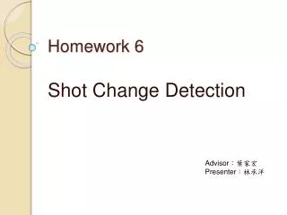
2. Chapter 4 Dynamical Behavior of Processes qi h1 h2 q1 qo a1 a2 v2 v1 Homework 6 • Construct an s-Function model of the interacting tank-in-series system and compare its simulation result with the simulation result of the component model from Homework 2. • For the tanks, use the same parameters as in Homework 2. • The required initial conditions are: h1,0 = 20 cm, h2,0 = 40 cm. • Deadline: The lecture session following the mid-term examination. • Send the softcopy and submit the hardcopy on time.

3. Chapter 4 Dynamical Behavior of Processes qi h1 h2 q1 qo a1 a2 v2 v1 Solution to Homework 6 • The interacting tank-in-series system can be described by these differential equation:

4. Chapter 4 Dynamical Behavior of Processes Solution to Homework 6

5. Chapter 4 Dynamical Behavior of Processes Solution to Homework 6 • Direct comparison between component model and s-function model

6. System Modeling and Identification Chapter 5 Discrete-Time Process Models

7. Chapter 5 Discrete-Time Process Models Computer-Controlled Systems • Computer-controlled system indicates that the control law is calculated by computer. • The feedback scheme of such system is shown below: A/D D/A : Digital-to-analog A/D : Analog-to-digital S/H : Sample-and-hold Ts: Sampling time, sampling period k : Integer, ≥ 0

8. Chapter 5 Discrete-Time Process Models Sampled Data System • The control error e(kTs) is given as the difference between the set point signal w(kTs) and the controlled process output y(kTs), in digital form, in times specified by the sampling period Ts. • The computer interprets the signal e(kTs) as a sequence of numbers and given the control law, it generates a new sequence of control signals u(kTs) • The discretized process represents a system with the input being the sequence of u(kTs) and the output being the sequence of y(kTs).

9. Chapter 5 Discrete-Time Process Models Classification of Signals • Continuous-time signals or analog signals: defined for every value of time they take on in a continuous interval (t0,t1). In other words, at any given instant an analog signal can take any value. For example, the signal x(t) = sin(t), − ∞ < t < ∞. • Discrete-time signals: defined only at specific values of time. These time instants need not be equidistant, but in practice they are usually taken at equally spaced intervals. In other words, the time variable of the signal can take only certain values. The amplitude of the signal can be continuous i.e., can take any value. For example, x(t) = sin(nt), n = 0,1,2,... n. • The process of converting an analog signal to discrete-time signal is called sampling. A discrete-time signal is sometimes called a sampled signal. • Discrete-valued signals or digital signal: arise when the discrete signals are quantized. A quantized signal assumes only discrete amplitude values. In other words, in these signals both the amplitude and time variable can take only certain values.

10. Chapter 5 Discrete-Time Process Models Classification of Signals • Digital grid of 0.1 : continuous-time signal (analog signal) : discrete-time signal (sampled signal) : discrete-valued signal (digital signal)

11. Chapter 5 Discrete-Time Process Models A/D Converter • The transformation of a continuous-time signal to a discrete-time signal is done by the A/D converter. A/D

12. Chapter 5 Discrete-Time Process Models D/A Converter • D/A converter with a sample-and-hold implements the transformation of a discrete-time signal to a continuous-time signal that is constant within one sampling period.

13. Chapter 5 Discrete-Time Process Models S/H Element • A possible realization of sample-and-hold is the zero-order hold with the transfer function of the form: • The sampling time Ts should be chosen in a way so that the process dynamics can be captured correctly. • High frequency continuous-time signals require high sampling frequency (fs), or equivalently, low sampling period Ts. • High frequency signal (cyan) and low frequency signal (gold) sampled with the same rate. • Same sample points are obtained.

14. Chapter 5 Discrete-Time Process Models Sampling Period • With small sampling period we may captures the dynamics of a system better, but the computational load will be heavier. • On the other hand, system with large sampling period may require low computational demand, but useful information might be lost. • In order to avoid loss of information but still capture the process dynamics correctly, the following inequality must hold: where Tsin is the lowest oscillation period of sinusoidal component of the sampled signal. • Nyquist-Shannon Sampling Theorem If a function x(t) contains no frequencies higher than β cycle-per-second, then it is completely determined by giving its ordinates at a series of points spaced 1/2β seconds apart.

15. Chapter 5 Discrete-Time Process Models Loss of Information Due To Sampling

16. Chapter 5 Discrete-Time Process Models Ideal Sampler • Let us now investigate properties of an ideal sampler. • Its output variable y* can be represented as a periodic sequence of δ functions as follows: • Representation in Fourier Series • Let us define ωs = 2π/Ts, and therefore

17. Chapter 5 Discrete-Time Process Models Ideal Sampler • The output variable of the ideal sampler can then be written as: • The Fourier transform of this function if y(0)=0 is given as:

18. Chapter 5 Discrete-Time Process Models Ideal Sampler • Substituting s for jω, Sum of series of original signal, shifted nωs away from the original frequency Sampling result = • The spectral density function of the variable y(t) is |Y(jω)|, while the spectral density of the sampled signal y*(t) is given as:

19. Chapter 5 Discrete-Time Process Models Ideal Sampler ωc : critical frequency ωs : sampling frequency Spectral density of original signal y(t) Spectral density of sampled signal y*(t)

20. Chapter 5 Discrete-Time Process Models ω –ωs 0 ωs Ideal Sampler • If ωc is smaller than or equal to half of the sampling frequency, the spectral density of |Y*(jω)| is composed of spectra of |Y(jω)| shifted to the right and left, nωs away. There are no overlapping. • If ωc is larger than half of the sampling frequency, then the spectral density of |Y*(jω)| consists of spectra |Y(jω)| shifted to the right and left, nωs away also. But now, there is overlapping. Hence the spectral density of the signal |Y*(jω)| is distorted. • If ωs < 2ωc, then overlapping occurs. • Original signal cannot be reconstructed from the sampled signal.

21. Chapter 5 Discrete-Time Process Models Choosing The Sampling Period • The sampling period choice is rather a problem of experience than some exact procedure. • Basically, sampling period has a strong influence on dynamic properties of the controlled system, as well as the whole closed-loop system. • The following rule of thumbs can be used to determine the sampling period of first- and second-order system: • 1st order τ/4 < Ts < τ/2 • 2nd order Tn/20 < Ts < Tn/4, Tn = 2π/ωn

22. Chapter 5 Discrete-Time Process Models Z-Transform • Let us again consider an ideal sampler, as shown below. • This sampler implements the transformation of a continuous-time signal f(t) to an impulse modulated signal f*(t). • Individual impulses appear on the sampler output in the sampling times kTs, k = 0, 1, 2, ... and are equal to functions f(kTs), k = 0, 1, 2, ... • This impulse modulated signal containing a sequence of impulses is denoted by f*(t), which can be expressed as: • The Laplace transform of this function is:

23. Chapter 5 Discrete-Time Process Models Z-Transform • Let us introduce a new variable • Then we can write • The Z-transform can now be defined as: • Z-transform is mathematically equivalent to Laplace transform and differs only in the argument. • Z-transform exists only if some z exists such that the series converges for k→∞.

24. Chapter 5 Discrete-Time Process Models Properties of Z-Transform • Shifting Theorem • Initial Value Theorem • Final Value Theorem • Given the Z-transform of a function, we can find the value of the function in time domain using the inverse Z-transform, but only for each value of sampled time, t = kTs.

25. Chapter 5 Discrete-Time Process Models Table of Z-Transform

26. Chapter 5 Discrete-Time Process Models Example Prove the table for the Z-transform of Recalling the formula to calculate the sum of infinite geometric series Then

27. Chapter 5 Discrete-Time Process Models Homework 7A Find the values y(kT) for k = 0 to 4, when We have a function Using a partial fraction expansion of Y(s) and the table given on previous slide, find Y(z) when Ts = 0.1 s.