Download
1 / 44
450 likes | 473 Views
Taxon Sampling for Ancestral State Reconstruction. Louxin Zhang Department of Mathematics Nat’l University of Singapore. Little Background to Ancestral Sequence Reconstruction . Ancestral sequence reconstruction incorporates sequences from modern organisms into evolutionary

E N D
Taxon Sampling for Ancestral State Reconstruction Louxin Zhang Department of Mathematics Nat’l University of Singapore
Little Background to Ancestral Sequence Reconstruction • Ancestral sequence reconstruction incorporates • sequences from modern organisms into evolutionary • models to estimate the corresponding sequence of • an ancestor that no longer presents on Earth. • This approach to understanding proteins or life in • general was proposed by Zuckerkandl and Pauling in 1963. • It has become an popular approach to studying • the origin, evolution, sequence-function relationship • of proteins, genes and other components of life.
After ~ 100 million years source: Carnegie Museum of Natural History How did we becomehuman? placental mammals
The differences are due to the changes in our DNA (Slide from J.Ma) human: ~3.1G, 23 chromosomes chimp: ~3.3G, 24 chromosomes mouse: ~2.7G, 20 chromosomes dog: ~2.5G, 39 chromosomes source: U.S. DOE
Recreate Genome of Ancient Human Ancestor • “Boreoeutherian ancestor” • lived 70 million yrs ago. • The boreoeutheria was formed • by a series of speciation events • occurring rapidly after the • ancestor, leading to • a star-like phylogeny of • boreoeutheria. • Computer simulation suggests • a small number of extant genomes • can give a highly accurate • reconstruction of this ancient • genomes. (Blanchette et al’04, Ma et al’07)
Ancestral State Reconstruction Problem • Given a phylogenetic tree T of a character - the evolutionary history of the character and an evolutionary model - prior distribution of all possible states at the root and substitution probability on each branch of T • Estimate the rootstate from the leaf states of the character in the tree T.
Part I: Methodsfor Ancestral State Reconstruction G A G A G G A G A G {G}U{ A} {G}U{ A} {G, A}∩{G} Fitch (parsimony) method Step 1: Compute a subset Sx of letters for each node x with children y and z as follows Step 2: Select a letter from the subset obtained at the root randomly. {G} ∩{G, A} G
Fitch method - It assigns a state to the root by minimizing the total number of substitutions placed on all branches -- It is a local and then efficient method. -- But, it ignores substitution rate on branches and is very sensitive to the topology of the tree, leading to several limitations
-- It is a global method and so less efficient. Approximation algs are studied. -- But, has the largest reconstruction accuracy, over all methods. Marginal maximum likelihood (ML) method - It assigns to the root a state a that has the maximum likelihood defined as Pr[ the root state is a| the given states at leaves ] and a tie is broken arbitrarily.
A Reconstruction Example Consider the following evolutionary model ( Tree + conservation rates + prior probabilities) for a character of two states 0 and 1. pprior(0)=pprior(1)=0.5 r 0.9 0.8 means that a state remains unchanged with probability 0.8. 0.8 0.9 0.9 0 1 1
For root state sr=0, 1 0 0 0 0.9 0.9 0.8 0.8 0.9 0.9 0.9 0.9 Pr[ 011 | sr=0 ] = 0.8x0.1x0.9x0.9 + 0.8x0.9x0.1x0.1=0.072 0 1 1 0 1 1
For root state sr=1, 1 0 1 1 0.9 0.9 0.8 0.8 0.9 0.9 0.9 0.9 0 1 1 0 1 1 Pr[ 011 | sr=1 ] = 0.2x0.9x0.9x0.9 + 0.2x0.1x0.1x0.1=0.1464
r pprior(0)=pprior(1)=0.5 0.9 0.8 Bayes formula: 0.9 0.9 0 1 1 Pr[ 011 | sr=0] = 0.072 Pr[ 011 | sr=1] = 0.1462 The marginal ML method selects 1 as the root state from leaves states 0 1 1.
Part II: Reconstruction Accuracy -- Definition For a reconstruction method M, its accuracy is the expected probability that the method reconstructs correctly the root state from a possible configuration D of states of leaf species: RAM( T ) = ∑c,DPr[c evolves into D] Pr[M reconstructs c from D] = ∑c,Dpprior(c) Pr[D|c] Pr [M reconstructs c from D]
{0} {0} {0, 1} {0, 1} {0} {0, 1} {1} {0} 0 0 0 0 0 1 0 1 1 1 0 0 Fitch selects 0 as the root state Fitch selects 0 as the root state Fitch selects 0 as the root state with prob 1/2 Fitch selects 0 as the root state with prob 1/2
Accuracy of Fitch method: pprior(0)=pprior(1)=0.5 RAF( T ) = ∑c,Dpprior(c) Pr[D|c] Pr [F reconstructs c from D] = ∑D Pr[D|0] Pr [F reconstructs 0 from D] = 0.584+0.072+0.072+0.146x0.5+0.072x0.5 = 0.837 r 0.9 Selected root state 0.8 Pr[D| sr = 1] Pr[D| sr = 0] 0.9 0.9 0 0 0 0.018 0.584 0 0 0 1 0.018 0.072 0 0 1 0 0.018 0.072 0 1 0 0 0.072 0.146 0 or 1(prob1/2) 0 1 1 0.146 0.072 0 or 1(prob1/2) 1 0 1 0.072 0.018 1 1 1 0 0.072 0.018 1 1 1 1 0.584 0.018 1
Accuracy of ML: pprior(0)=pprior(1)=0.5 RAML( T ) = ∑c,Dpprior(c) Pr[D|c] Pr [ML reconstructs c from D] = ∑D Pr[D|0] Pr [ML reconstructs 0 from D] = 0.584+0.072 + 0.072 + 0.146 = 0.874 r 0.9 Selected root state 0.8 Pr[D| sr = 1] Pr[D| sr = 0] 0.9 0.9 0 0 0 0.018 0.584 0 0 0 1 0.018 0.072 0 0 1 0 0.018 0.072 0 1 0 0 0.072 0.146 0 0 1 1 0.146 0.072 1 1 0 1 0.072 0.018 1 1 1 0 0.072 0.018 1 1 1 1 0.584 0.018 1
Forthe ML method and tree H, RAML( H ) = ∑c,DPr[c evolves into D] Pr[MLreconstructs c from D] = ∑D∑cPr[c evolves into D] Pr[ML reconstructs c from D] = ∑Dmaxc Pr[c evolves into D] c D: A G C G G
Part II: Reconstruction Accuracy -- Monotonicity When reconstructing the state of the common ancestor for a group of organisms, one would expect that the accuracy will increase with the number of organisms used. However, this is not always true over a phylogeny for a method? In other words, more organisms do not necessarily give better estimation for ancestral state.
Theorem: The accuracy function of the Fitch method is not monotonic. Consider the following tree (Li, Steel, Zhang’08) r pprior(a)=pprior(b)=0.5 0.8 0.9 0.9 0.9 The accuracy of reconstruction from all leaves is 0.866, while the accuracy of reconstruction from the left leaf is 0.9 Does this counterintuitive fact occur often?
A counterexample with ultrametric tree in which the root is equally far from all leaves. The accuracy of reconstruction from all leaves is 0.915268; the accuracy of reconstruction from a, i, b, e is 0.921926 14.1190 10.0613 9.7109 24.9926 17.5103 21.7263 47.8447 50.0000
More taxa are not necessarily good in ancestral sequence reconstruction when the Fitch method is applied. More sequences data do not always lead to the true phylogeny when the parsimony method is used. There are probably two reasons for these counterintuitive facts -- It ignores character change rate on all branches; -- the Fitch method is a kind of ‘local method’ .
Theorem: The maximum likelihood (ML) method has the largest reconstructing accuracy over all methods for any tree and evolution model. Corollary: The accuracy function of the ML method is monotonic Proof of Corollary. -- Using a subset of leaves is just a specific reconstruction method that does not use letter information in the other leaves -- hence its accuracy is not higher than the reconstruction from all the leaves when ML is used.
Proof of Theorem: For any method M and tree H, RAM( H ) = ∑c,DPr[c evolves into D] Pr[M reconstructs c from D] = ∑D∑cPr[c evolves into D] Pr[M reconstructs c from D] ≤ ∑D∑c(maxc Pr[c evolves into D]) Pr[M reconstructs c from D] = ∑D (maxc Pr[c evolves into D]) {∑c Pr[M reconstructs c from D]} = ∑D (maxc Pr[c evolves into D]) = RAML( H ) c D: A G C G G
Part III: Reconstruction Accuracy -- Computation Is the reconstruction accuracy RAM(T) polynomial-time computable for any phylogeny T , given a simple Markovian evolutionary model (say, Juke-Cantor ) and a method M?
Theorem: The reconstruction accuracy is linear-time computable for Fitch method. Proof : r Z Y X
Computing the accuracy of ML Theorem 1 (B. Ma & Zhang’09). For any n-leaf tree T in which a binary character changes with probability at most q<1/2 on each branch, RAML(T) can be approximated within ratio 1- ε in O(n N4) for any ε, where N= It is unknown how to compute the accuracy of ML in polynomial time.
Some notations r : the root of tree T; D: state configuration of leaves; pprior(a): the prior probability of a root state a; Pr[ D | sr=a]: the probability that root state a evolves into states in D; Pr [ sr =a | D]: the probability that the root state is a given that states in D are observed in leaves. It is called likelihood of the state given D.
State c can evolve into D in 2k-2 ways. For • each way E, Lemma 1. Let T be phylogeny of k (>1) leaves with root r. For any configuration D of leaves of T and c, Proof. It is based on the following facts: (1) T has 2(k-1) edges;
Method Summary RAML(T)= -- Discretize the probability space x0=q2(n-1) , xi+1 = xi/(1-ε) 1/(n-1), i<N; xN=1 --- Calculate the sum of the estimates of the mutational probability recursively.
Remarks • Our approach is superior to the sampling • approach since it can also be used to estimate • efficiently the reconstruction error rate. • Both computing the accuracy and the error • rate for ML method have unknown complexity • status. • Are they NP-hard?
Part IV: Reconstruction Accuracy -- Taxon Selection -- Fitch method is efficient, but does not monotonic accuracy ; -- ML method has monotonic accuracy, but computationally intensive K-Taxa Selection Problem: Input: An evolutionary model ( A tree + substitution rate on branches), a method M, and an integer k>0; Objective: Find k taxa from which the root state can be reconstructed with the highest accuracy when M is used.
Question: Is the K-Taxa Selection Problem NP-hard? For Fitch method, the bucket idea can be used to give a good approximation to the K-taxa selection problem (E. Mossel’08) Question: How to generalize bucket idea to study the K-Species Selection Problem for ML method?
Performance comparison The accuracy of reconstruction from all taxa - the accuracy of reconstruction from a selected subset of taxa Performance on the greedy algorithms on random trees with 16 leaves in a Yule model
Performance comparison The accuracy of reconstruction from all taxa - the accuracy of reconstruction from a selected subset of taxa Performance on the greedy algorithms on random ultrametric trees
DNA Sequence data: Estimating Boreoeutherian Seq ( from Adam Siepel)
Lessons learnt from our experiments -- The backward greedy selection outperforms the forward greedy selection. -- When the small number (<10) of taxa are used, the reconstruction accuracy varies in a wide range especially for the Fitch method. This large variability of accuracy indicates that caution should be exercised in drawing conclusions on an ancestral sequence reconstructed from a small number of taxa. -- With around 15 organisms, the boreoeutherian ancestral sequence can be reconstruction with high resolution.
Summary Fitch method Maximum Likelihood Monotonicity of the accuracy No Yes Computing the accuracy Linear-time algorithm Good poly-time approx. alg. NP? Taxon selection problem Good poly-time approx. alg. ? NP? NP? Backward Selection Method Future Work: Extend our work to general evolution models where more evolutionary events are considered
Acknowledgement Guoling Li Genome Institute of Singapore Jian Ma UC Santa Cruz, USA Bin Ma University of Waterloo , Canada Mike Steel University of Canterbury, New Zealand