Download
1 / 23
230 likes | 332 Views
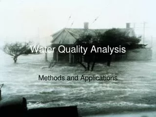
Introduction to the Water Quality Analysis Modeling System. WASP Version 7.0 April, 2005. US EPA Disclaimer. Although this work was reviewed by EPA and approved for presentation, it may not necessarily reflect official Agency policy.

E N D
Introduction to the Water Quality Analysis Modeling System WASP Version 7.0 April, 2005 WASP 7 Course
US EPA Disclaimer Although this work was reviewed by EPA and approved for presentation, it may not necessarily reflect official Agency policy. Mention of trade names or commercial products does not constitute endorsement or recommendation for use. WASP 7 Course
Course Objectives • Modeling Principles • Modeling Theory • Processes in WASP • Limitations of process descriptions • Modeling Practice • Using the WASP Interface • Using WASP for real-world problems • Case Study Applications of WASP • Discussion of Data Needs WASP 7 Course
Basic Principle of Mechanistic Models • Laws of Conservation • Conservative properties are those that are not gained or lost through ordinary reactions. Therefore we can account for any change by simply keeping track of all those processes that can cause change • Examples of conservative properties • Mass (water mass, constituent mass) • Momentum • Heat WASP 7 Course
Control Volume z y x Three Dimensional Transport Equation WASP 7 Course
Box Model Approach • Numerical solution allows greater flexibility as to processes considered (i.e. eutrophication, toxics, etc.) • Allows greater flexibility as to segmentation • Flows and mixing coefficients are obtained from • Field data • Hydrodynamic models (which produce output that can be read by WASP) WASP 7 Course
Box Modeling Approach • Boxes • The boxes have no defined shape, so can be fit to any morphometry • The boxes can be “stacked” so the approach can be applied to 0 dimensions (1 box) or 1, 2 or three dimensional systems WASP 7 Course
WASP Modeling Framework Model Preprocessor/Data Server Binary Wasp Input File (wif) CSV, ASCII Output WASP Input Messages Models Hydrodynamic Interface BinaryModelOutput Stored Data BMD Eutrophication Hydro Conservative Toxicant ExportedModelResults Organic Toxicants MOVEM Mercury Graphical Post Processor Heat WASP 7 Course
WASP7 Water Quality Modules • Eutrophication (eutro.dll) • DO, BOD, nutrients, phytoplankton, periphyton • Simple Toxicant (toxi.dll) • Partitioning and first order decay • Simple metal or organic chemical, solids • Non-Ionic Organic Toxicants (toxi.dll) • Detailed fate processes, reaction products, solids • Organic Toxicants (toxi.dll) • Detailed fate processes, ionization, reaction products, solids • Mercury (mercury.dll), slightly altered from toxi.dll • Hg0, HgII, MeHg, solids • HEAT (heat.dll) • full/equilibrium heat balance + pathogens WASP 7 Course
WASP Structure WASP Transport Bookkeeping Organic Chemical Model Eutrophication Model Mercury Model Kinetics WASP 7 Course
1 2 3 4 5 6 NH3 NO3 DO BOD Chla OPO4 Systems (i.e., State Variables) Calculated Variables BOD Decay Rate Growth Rate, etc. WASP Terminology Segments WASP 7 Course
EUTRO Dissolved oxygen CBOD (three forms) Phytoplankton Periphyton Detritus (C, N, P) Dissolved organic nitrogen Ammonia/ammonium Nitrate Dissolved organic phosphorus Orthophosphate Salinity Solids Sediment Diagenesis WASP Systems: Conventional Water Quality Modules • HEAT • Temperature • Salinity • Coliform • Conservative 1 and 2 WASP 7 Course
Simple Toxicant Chemical Silts/Fines Sands Biotic solids Organic Toxicants (both non-ionizing and ionizing) Chemical 1 Chemical 2 Chemical 3 Silts/Fines Sands Biotic solids WASP Systems: Toxicant Modules • Mercury • Elemental, Hg0 • Divalent, HgII • Methyl, MeHg • Silts/Fines • Sands • Biotic solids WASP 7 Course
Potential WASP Time Scales • Steady • Seasonal • Monthly • Daily/Hourly WASP 7 Course
WASP Advantages and Features • Network Flexibility • Applicable to most water body types at some level of complexity • Most Water Quality Problems • Conventional Water Quality: DO, eutrophication, heat • Toxicant Fate: organics, simple metals, mercury • Separation of Processes • Transport • Kinetics • External Links to Models and Spreadsheets • Two Solution Techniques • Simple/Quick – Euler • Complex/Flux Limiting -- COSMIC WASP 7 Course
WASP External Linkages Loading Models SWMM HSPF LSPC NPSM PRZM GBMM Bioaccumulation BASS FCM-2 WASP Hydrodynamic Models EFDC DYNHYD EPD-RIV1 SWMM External Spreadsheets ASCII Files Windows Clipboard WASP 7 Course
WASP Limitations • Does not handle some variables and processes: • Mixing zone processes • Non aqueous phase liquids (e.g., oil spills) • Segment drying (mudflats, flood plains) • Metals speciation reactions (special module, META4, not part of general WASP release) • Potentially large external hydrodynamic files • Separate eutrophication and toxicant fate modules • Cannot readily be run in batch mode • Automatic calibration programs • Monte Carlo programs WASP 7 Course
WASP is a Variable Complexity Modeling System • When building a water body model, adjust complexity to match the problem. • More Complex Aquatic Systems • More Complex Chemical Behavior • More Complex Management Questions WASP 7 Course
A model is more like a than a Dominic Di Toro Development of Complexity in Water Quality ModelingApplications WASP 7 Course
General Conceptual Model Available Data Site-Specific Conceptual Model (Preliminary Data Collection) Initial Screening Mathematical Model (usually simple) Project Data Collection Evolving Operational Mathematical Model (usually more complex) Model evaluation, Post-audit data Iterative Model Development Process WASP 7 Course
How Complex Should Final Computational Model Be? • Proper model complexity is driven by: • The complexity of the environmental system. • The complexity of the pollutants of concern. • The management questions and related need for accuracy. • Consequences for overly simple model: • Miss key processes and extrapolate inaccurately. • May not address relevant management questions. • May not be defensible to adversarial review. • Insufficiently adaptable to changing management requirements. • Consequences for overly complex model: • Adds unnecessary data collection and computational burdens. • Adds to uncertainty. • Shifts focus away from problem solutions to endless analysis. WASP 7 Course
Management-Related Questions Requiring More Complex Models • What are the spatial and temporal distributions of target pollutants (particularly in mixed-media environments) under various management scenarios? • What are the relative contributions of various sources of pollutants over time? • What are the likely pollutant attenuation trajectories and times to recovery under various management scenarios? • What are the relative effects of transient or extreme events, such as spills or storms? • What are the possible effects of poorly understood environmental events? WASP 7 Course
“Make things as simple as possible, but not any simpler.” Albert Einstein Goal of Model Complexity WASP 7 Course