Download
1 / 44
440 likes | 446 Views
Introduction Concurrent Programming Communication and Synchronization Completing the Java Model Overview of the RTSJ Memory Management Clocks and Time. Scheduling and Schedulable Objects Asynchronous Events and Handlers Real-Time Threads Asynchronous Transfer of Control

E N D
Introduction Concurrent Programming Communication and Synchronization Completing the Java Model Overview of the RTSJ Memory Management Clocks and Time Scheduling and Schedulable Objects Asynchronous Events and Handlers Real-Time Threads Asynchronous Transfer of Control Resource Control Schedulability Analysis Conclusions Roadmap
Scheduling • Lecture aims • To understand the role that scheduling and schedulability analysis plays in predicting that real-time applications meet their deadlines • Education onlu - not examinable • Topics • Simple process model • The cyclic executive approach • Process-based scheduling • Utilization-based schedulability tests • Response time analysis for FPS and EDF • Worst-case execution time • Sporadic and aperiodic processes • Process systems with D < T • Process interactions, blocking and priority ceiling protocols • Dynamic systems and on-line analysis
Scheduling • In general, a scheduling scheme provides two features: • An algorithm for ordering the use of system resources (in particular the CPUs) • A means of predicting the worst-case behaviour of the system when the scheduling algorithm is applied • The prediction can then be used to confirm the temporal requirements of the application
Simple Process Model • The application is assumed to consist of a fixed set of processes • All processes are periodic, with known periods • The processes are completely independent of each other • All system's overheads, context-switching times and so on are ignored (i.e, assumed to have zero cost) • All processes have a deadline equal to their period (that is, each process must complete before it is next released) • All processes have a fixed worst-case execution time
B C D I N P R T U a-z Worst-case blocking time for the process (if applicable) Worst-case computation time (WCET) of the process Deadline of the process The interference time of the process Number of processes in the system Priority assigned to the process (if applicable) Worst-case response time of the process Minimum time between process releases (process period) The utilization of each process (equal to C/T) The name of a process Standard Notation
Cyclic Executives • One common way of implementing hard real-time systems is to use a cyclic executive • Here the design is concurrent but the code is produced as a collection of procedures • Procedures are mapped onto a set of minor cycles that constitute the complete schedule (or major cycle) • Minor cycle dictates the minimum cycle time • Major cycle dictates the maximum cycle time Has the advantage of being fully deterministic
Properties • No actual processes exist at run-time; each minor cycle is just a sequence of procedure calls • The procedures share a common address space and can thus pass data between themselves. This data does not need to be protected (via a semaphore, for example) because concurrent access is not possible • All “process” periods must be a multiple of the minor cycle time
Problems with Cycle Executives • The difficulty of incorporating processes with long periods; the major cycle time is the maximum period that can be accommodated without secondary schedules • Sporadic activities are difficult (impossible!) to incorporate • The cyclic executive is difficult to construct and difficult to maintain — it is a NP-hard problem • Any “process” with a sizable computation time will need to be split into a fixed number of fixed sized procedures (this may cut across the structure of the code from a software engineering perspective, and hence may be error-prone) • More flexible scheduling methods are difficult to support • Determinism is not required, but predictability is
Process-Based Scheduling • Scheduling approaches • Fixed-Priority Scheduling (FPS) • Earliest Deadline First (EDF) • Value-Based Scheduling (VBS)
Fixed-Priority Scheduling (FPS) • This is the most widely used approach and is the main focus of this course • Each process has a fixed, static, priority which is computer pre-run-time • The runnable processes are executed in the order determined by their priority • In real-time systems, the “priority” of a process is derived from its temporal requirements, not its importance to the correct functioning of the system or its integrity
FPS and Rate Monotonic Priority Assignment • Each process is assigned a (unique) priority based on its period; the shorter the period, the higher the priority • I.e, for two processes i and j, • This assignment is optimal in the sense that if any process set can be scheduled (using pre-emptive priority-based scheduling) with a fixed-priority assignment scheme, then the given process set can also be scheduled with a rate monotonic assignment scheme • Note, priority 1 is the lowest (least) priority
Example Priority Assignment Process Period, T Priority, P a 25 5 b 60 3 c 42 4 d 105 1 e 75 2
Utilisation-Based Analysis • For D=T task sets only • A simple sufficient but not necessary schedulability test exists
Utilization Bounds N Utilization bound 1 100.0% 2 82.8% 3 78.0% 4 75.7% 5 74.3% 10 71.8% Approaches 69.3% asymptotically
Process Set A • The combined utilization is 0.82 (or 82%) • This is above the threshold for three processes (0.78) and, hence, this process set fails the utilization test Process Period ComputationTime Priority Utilization T C P U a 50 12 1 0.24 b 40 10 2 0.25 c 30 10 3 0.33
0 10 20 30 40 50 60 Time-line for Process Set A Process a Process Release Time Process Completion Time Deadline Met b Process Completion Time Deadline Missed Preempted c Executing Time
Gantt Chart for Process Set A c b a c b 0 10 20 30 40 50 Time
Process Set B • The combined utilization is 0.775 • This is below the threshold for three processes (0.78) and, hence, this process set will meet all its deadlines Process Period ComputationTime Priority Utilization T C P U a 80 32 1 0.400 b 40 5 2 0.125 c 16 4 3 0.250
Process Set C • The combined utilization is 1.0 • This is above the threshold for three processes (0.78) but the process set will meet all its deadlines Process Period ComputationTime Priority Utilization T C P U a 80 40 1 0.50 b 40 10 2 0.25 c 20 5 3 0.25
0 10 20 30 40 50 60 Time-line for Process Set C Process a b c 70 80 Time
Criticism of Utilisation-based Tests • Not exact • Not general • BUT it is O(N) The test is said to be sufficient but not necessary
Response-Time Analysis • Here task i's worst-case response time, R, is calculated first and then checked (trivially) with its deadline R D i i Where I is the interference from higher priority tasks
Calculating R During R, each higher priority task j will execute a number of times: The ceiling function gives the smallest integer greater than the fractional number on which it acts. So the ceiling of 1/3 is 1, of 6/5 is 2, and of 6/3 is 2. Total interference is given by:
Solve by forming a recurrence relationship: The set of values is monotonically non decreasing When the solution to the equation has been found, must not be greater that (e.g. 0 or ) Response Time Equation Where hp(i) is the set of tasks with priority higher than task i
Process Set D Process Period ComputationTime Priority T C P a 7 3 3 b 12 3 2 c 20 5 1
Revisit: Process Set C Process Period ComputationTime Priority Response time T C P R a 80 40 1 80 b 40 10 2 15 c 20 5 3 5 • The combined utilization is 1.0 • This was above the ulilization threshold for three processes (0.78), therefore it failed the test • The response time analysis shows that the process set will meet all its deadlines • RTA is necessary and sufficient
Response Time Analysis • Is sufficient and necessary • If the process set passes the test they will meet all their deadlines; if they fail the test then, at run-time, a process will miss its deadline (unless the computation time estimations themselves turn out to be pessimistic)
Worst-Case Execution Time - WCET • Obtained by either measurement or analysis • The problem with measurement is that it is difficult to be sure when the worst case has been observed • The drawback of analysis is that an effective model of the processor (including caches, pipelines, memory wait states and so on) must be available
WCET— Finding C Most analysis techniques involve two distinct activities. • The first takes the process and decomposes its code into a directed graph of basic blocks • These basic blocks represent straight-line code • The second component of the analysis takes the machine code corresponding to a basic block and uses the processor model to estimate its worst-case execution time • Once the times for all the basic blocks are known, the directed graph can be collapsed
Need for Semantic Information for I in 1.. 10 loop if Cond then -- basic block of cost 100 else -- basic block of cost 10 end if; end loop; • Simple cost 10*100 (+overhead), say 1005. • But if Cond only true on 3 occasions then cost is 375
Sporadic Processes • Sporadics processes have a minimum inter-arrival time • They also require D<T • The response time algorithm for fixed priority scheduling works perfectly for values of D less than T as long as the stopping criteria becomes • It also works perfectly well with any priority ordering — hp(i) always gives the set of higher-priority processes
Hard and Soft Processes • In many situations the worst-case figures for sporadic processes are considerably higher than the averages • Interrupts often arrive in bursts and an abnormal sensor reading may lead to significant additional computation • Measuring schedulability with worst-case figures may lead to very low processor utilizations being observed in the actual running system
General Guidelines Rule 1— all processes should be schedulable using average execution times and average arrival rates Rule 2— all hard real-time processes should be schedulable using worst-case execution times and worst-case arrival rates of all processes (including soft) • A consequent of Rule 1 is that there may be situations in which it is not possible to meet all current deadlines • This condition is known as a transientoverload • Rule 2 ensures that no hard real-time process will miss its deadline • If Rule 2 gives rise to unacceptably low utilizations for “normal execution” then action must be taken to reduce the worst-case execution times (or arrival rates)
Aperiodic Processes • These do not have minimum inter-arrival times • Can run aperiodic processes at a priority below the priorities assigned to hard processes, therefore, they cannot steal, in a pre-emptive system, resources from the hard processes • This does not provide adequate support to soft processes which will often miss their deadlines • To improve the situation for soft processes, a server can be employed. • Servers protect the processing resources needed by hard processes but otherwise allow soft processes to run as soon as possible. • POSIX supports Sporadic Servers
Process Sets with D < T • For D = T, Rate Monotonic priority ordering is optimal • For D < T, Deadline Monotonic priority ordering is optimal
D < T Example Process Set Process Period Deadline ComputationTime Priority Response time T D C P R a 20 5 3 4 3 b 15 7 3 3 6 c 10 10 4 2 10 d 20 20 3 1 20
Process Interactions and Blocking • If a process is suspended waiting for a lower-priority process to complete some required computation then the priority model is, in some sense, being undermined • It is said to suffer priority inversion • If a process is waiting for a lower-priority process, it is said to be blocked
Dynamic Systems and Online Analysis • There are dynamic soft real-time applications in which arrival patterns and computation times are not known a priori • Although some level of off-line analysis may still be applicable, this can no longer be complete and hence some form of on-line analysis is required • The main task of an on-line scheduling scheme is to manage any overload that is likely to occur due to the dynamics of the system's environment • EDF is a dynamic scheduling scheme that is an optimal • During transient overloads EDF performs very badly. It is possible to get a cascade effect in which each process misses its deadline but uses sufficient resources to result in the next process also missing its deadline
Admission Schemes • To counter this detrimental domino effect, many on-line schemes have two mechanisms: • an admissions control module that limits the number of processes that are allowed to compete for the processors, and • an EDF dispatching routine for those processes that are admitted • An ideal admissions algorithm prevents the processors getting overloaded so that the EDF routine works effectively
Values • If some processes are to be admitted, whilst others rejected, the relative importance of each process must be known • This is usually achieved by assigning value • Values can be classified • Static: the process always has the same value whenever it is released. • Dynamic: the process's value can only be computed at the time the process is released (because it is dependent on either environmental factors or the current state of the system) • Adaptive: here the dynamic nature of the system is such that the value of the process will change during its execution • To assign static values requires the domain specialists to articulate their understanding of the desirable behaviour of the system
Summary • A scheduling scheme defines an algorithm for resource sharing and a means of predicting the worst-case behaviour of an application when that form of resource sharing is used. • With a cyclic executive, the application code must be packed into a fixed number of minor cycles such that the cyclic execution of the sequence of minor cycles (the major cycle) will enable all system deadlines to be met • The cyclic executive approach has major drawbacks many of which are solved by priority-based systems • Simple utilization-based schedulability tests are not exact
Summary • Response time analysis is flexible and caters for: • Periodic and sporadic processes • Blocking caused by IPC • Cooperative scheduling (not covered) • Arbitrary deadlines (not covered) • Release jitter (not covered) • Fault tolerance (not covered) • Offsets (not covered) • RT Java supports preemptive priority-based scheduling • RT Java addresses dynamic systems with the potential for on-line analysis