Download
1 / 48
1.23k likes | 2.75k Views
Chapter 10: Image Segmentation. Digital Image Processing. Preview. Segmentation is to subdivide an image into its component regions or objects. Segmentation should stop when the objects of interest in an application have been isolated. Principal approaches.

E N D
Chapter 10: Image Segmentation Digital Image Processing
Preview • Segmentation is to subdivide an image into its component regions or objects. • Segmentation should stop when the objects of interest in an application have been isolated.
Principal approaches Segmentation algorithms generally are based on one of 2 basis properties of intensity values discontinuity : to partition an image based on sharp changes in intensity (such as edges) similarity : to partition an image into regions that are similar according to a set of predefined criteria.
Detection of Discontinuities • detect the three basic types of gray-level discontinuities • points , lines , edges • the common way is to run a mask through the image
Point Detection • a point has been detected at the location on which the mark is centered if |R| T • where • T is a nonnegative threshold • R is the sum of products of the coefficients with the gray levels contained in the region encompassed by the mark.
Point Detection • Note that the mark is the same as the mask of Laplacian Operation (in chapter 3) • The only differences that are considered of interest are those large enough (as determined by T) to be considered isolated points. |R| T
Line Detection • Horizontal mask will result with max response when a line passed through the middle row of the mask with a constant background. • the similar idea is used with other masks. • note: the preferred direction of each mask is weighted with a larger coefficient (i.e.,2) than other possible directions.
Line Detection • Apply every masks on the image • let R1, R2, R3, R4 denotes the response of the horizontal, +45 degree, vertical and -45 degree masks, respectively. • if, at a certain point in the image |Ri| > |Rj|, • for all ji, that point is said to be more likely associated with a line in the direction of mask i.
Line Detection • Alternatively, if we are interested in detecting all lines in an image in the direction defined by a given mask, we simply run the mask through the image and threshold the absolute value of the result. • The points that are left are the strongest responses, which, for lines one pixel thick, correspond closest to the direction defined by the mask.
Edge Detection • we discussed approaches for implementing • first-order derivative (Gradient operator) • second-order derivative (Laplacian operator) • Here, we will talk only about their properties for edge detection. • we have introduced both derivatives in chapter 3
because of optics, sampling, image acquisition imperfection Ideal and Ramp Edges
Thick edge • The slope of the ramp is inversely proportional to the degree of blurring in the edge. • We no longer have a thin (one pixel thick) path. • Instead, an edge point now is any point contained in the ramp, and an edge would then be a set of such points that are connected. • The thickness is determined by the length of the ramp. • The length is determined by the slope, which is in turn determined by the degree of blurring. • Blurred edges tend to be thick and sharp edges tend to be thin
the signs of the derivatives would be reversed for an edge that transitions from light to dark First and Second derivatives
Second derivatives • produces 2 values for every edge in an image (an undesirable feature) • an imaginary straight line joining the extreme positive and negative values of the second derivative would cross zero near the midpoint of the edge. (zero-crossing property)
Zero-crossing • quite useful for locating the centers of thick edges • we will talk about it again later
Noise Images • First column: images and gray-level profiles of a ramp edge corrupted by random Gaussian noise of mean 0 and = 0.0, 0.1, 1.0 and 10.0, respectively. • Second column: first-derivative images and gray-level profiles. • Third column : second-derivative images and gray-level profiles.
Keep in mind • fairly little noise can have such a significant impact on the two key derivatives used for edge detection in images • image smoothing should be serious consideration prior to the use of derivatives in applications where noise is likely to be present.
Edge point • to determine a point as an edge point • the transition in grey level associated with the point has to be significantly stronger than the background at that point. • use threshold to determine whether a value is “significant” or not. • the point’s two-dimensional first-order derivative must be greater than a specified threshold.
commonly approx. the magnitude becomes nonlinear Gradient Operator • first derivatives are implemented using the magnitude of the gradient.
Laplacian operator (linear operator) Laplacian
where r2 = x2+y2, and is the standard deviation Laplacian of Gaussian • Laplacian combined with smoothing to find edges via zero-crossing.
positive central term surrounded by an adjacent negative region (a function of distance) zero outer region Mexican hat the coefficient must be sum to zero
Linear Operation • second derivation is a linear operation • thus, 2f is the same as convolving the image with Gaussian smoothing function first and then computing the Laplacian of the result
Example a). Original image b). Sobel Gradient c). Spatial Gaussian smoothing function d). Laplacian mask e). LoG f). Threshold LoG g). Zero crossing
Zero crossing & LoG • Approximate the zero crossing from LoG image • to threshold the LoG image by setting all its positive values to white and all negative values to black. • the zero crossing occur between positive and negative values of the thresholded LoG.
Thresholding image with dark background and a light object image with dark background and two light objects
Multilevel thresholding • a point (x,y) belongs to • to an object class if T1 < f(x,y) T2 • to another object class if f(x,y) > T2 • to background if f(x,y) T1 • T depends on • only f(x,y) : only on gray-level values Global threshold • both f(x,y) and p(x,y) : on gray-level values and its neighbors Local threshold
easily use global thresholding object and background are separated The Role of Illumination f(x,y) = i(x,y) r(x,y) a). computer generated reflectance function b). histogram of reflectance function c). computer generated illumination function (poor) d). product of a). and c). e). histogram of product image difficult to segment
use T midway between the max and min gray levels generate binary image Basic Global Thresholding
Basic Global Thresholding • based on visual inspection of histogram • Select an initial estimate for T. • Segment the image using T. This will produce two groups of pixels: G1 consisting of all pixels with gray level values > T and G2 consisting of pixels with gray level values T • Compute the average gray level values 1 and 2 for the pixels in regions G1 and G2 • Compute a new threshold value • T = 0.5 (1 + 2) • Repeat steps 2 through 4 until the difference in T in successive iterations is smaller than a predefined parameter To.
Example: Heuristic method note: the clear valley of the histogram and the effective of the segmentation between object and background T0 = 0 3 iterations with result T = 125
Basic Adaptive Thresholding • subdivide original image into small areas. • utilize a different threshold to segment each subimages. • since the threshold used for each pixel depends on the location of the pixel in terms of the subimages, this type of thresholding is adaptive.
Further subdivision a). Properly and improperly segmented subimages from previous example b)-c). corresponding histograms d). further subdivision of the improperly segmented subimage. e). histogram of small subimage at top f). result of adaptively segmenting d).
Boundary Characteristic for Histogram Improvement and Local Thresholding light object of dark background • Gradient gives an indication of whether a pixel is on an edge • Laplacian can yield information regarding whether a given pixel lies on the dark or light side of the edge • all pixels that are not on an edge are labeled 0 • all pixels that are on the dark side of an edge are labeled + • all pixels that are on the light side an edge are labeled -
Region-Based Segmentation - Region Growing • start with a set of “seed” points • growing by appending to each seed those neighbors that have similar properties such as specific ranges of gray level
select all seed points with gray level 255 Region Growing • criteria: • the absolute gray-level difference between any pixel and the seed has to be less than 65 • the pixel has to be 8-connected to at least one pixel in that region (if more, the regions are merged)