Download
1 / 13
140 likes | 242 Views
Numerical Hydraulics. Lecture 4: Computation of pressure surges continued. W. Kinzelbach with Marc Wolf and Cornel Beffa. Additions. Formation of vapour bubble Branching pipes Different closing functions Pumps and pressure reduction valves ….

E N D
Numerical Hydraulics Lecture 4: Computation of pressure surges continued W. Kinzelbach with Marc Wolf and Cornel Beffa
Additions • Formation of vapour bubble • Branching pipes • Different closing functions • Pumps and pressure reduction valves • …. • Consistent initial conditions through steady state computation of flow/pressure distribution
t or Q (%) 100 0 0 tclose time t closed open Closing function • Expressed as Q=Q(t) or by degree of closure t, depending from position of valve, t = f(t) • Valve closed: t = 0 • Valve completely open: t = 1 • In between: function corresponding to ratio of loss coefficients Index 0 refers to open valve
Valve as boundary condition • Valve directly in front of a downstream reservoir with pressure pB2 • Valve at Node N+1 • Linear closing function t = 1-t/tclose • Determine new pressure and velocity at valve For t < tclose: From boundary condition (1) From forward characteristic (2) Inserting (1) into (2) yields quadratic equation for
Valve as boundary condition Only one of the two solutions is physically meaningful For t > tclose:
Pump Given characteristic function of pump: Pump at node i: Simply insert into characteristic equation. e.g. forward characteristic:
Formation of vapour bubble If the pressure falls below the vapour pressure of the fluid (at temperature T) a vapour bubble forms, which fixes the pressure at the vapour pressure of the fluid. The bubble grows as long as the pressure in the fluid does not rise. It collapses again when the pressure increases above the vapour pressure. As long as the vapour bubble exists, the boundary condition v = 0 at the valve must be replaced by the pressure boundary condition p = pvapour . Additional equation: Forward characteristic in N: Volume balance of vapour bubble: volume Vol at valve If Vol becomes 0 the vapour bubble has collapsed. The velocity in the volume equation is negative, as bubble grows as long as wave moves away from valve.
Branching of pipe k+1 k i+1 i-1 i Characteristics along i -1 … k+1 and along i -1 … i+1 Note that continuity requires that Ai-1vi-1=Akvk+Aivi With different lengths of pipes the reflected waves return at different times. At the branching, partial reflection takes place. The pressure surge signal in a pipe grid therefore becomes much more complicated, but at the same time less extreme, as the interferences weaken the maximum.
Tank 2 Tank 1 connecting pipe Consistent initial conditions by steady state computation of flow/pressure In the example: In a grid with branchings a steady state computation of the whole grid is required
Measures against pressure surges • Slowing down of closing process • Surge vessel (Windkessel) • Surge shaft • Special valves air
Surge shaft oscillations Task: Write a program in Matlab for the calculation of the surge shaft oscillations Simplified theory: see next page
Surge shaft oscillations • The following formulae can be used (approximation of rigid water column) : Solve for Z(t), Estimate the frequency under neglection of friction. Data: l = 200 m, d1 = 1.25 m, d2 = 4 m, Q = 2 m3/s at time t = 0 local losses negligible, l = 0.04, computation time from t = 0 to t = 120 s, instantaneous closing of valve at time t = 0.
Surge shaft oscillations The surge in the following surge shaft is to be calculated using the program Hydraulic System. Vary parameters and compare! w stands for wall thickness, in the pressure duct in the rock it is assumed as 2 m effectively. 250 m ü. M. Further data: Closing time 1 s, area surge shaft 95 m2, roughness pressure duct k=0.00161 m, modulus of elasticity pressure duct = 30 GN/m2, modulus of elasticity pressure duct = 30 GN/m2, Loss coefficient valve 2.1 (am ->av) and 2.0 (am<- av) resp., linear closing law, cross-section valve 1.5 m