5.2. Observations of convectively coupled KWs

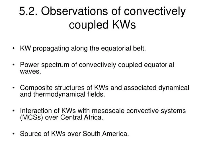
1. 5.2. Observations of convectively coupled KWs • KW propagating along the equatorial belt. • Power spectrum of convectively coupled equatorial waves. • Composite structures of KWs and associated dynamical and thermodynamical fields. • Interaction of KWs with mesoscale convective systems (MCSs) over Central Africa. • Source of KWs over South America.

2. Kelvin wave over the Pacific warm pool Movie of CLAUS Tb in May 1998

3. Kelvin wave over the Amazon Movie of CLAUS Tb in May 1998

4. Kelvin wave over equatorial Africa Movie of CLAUS Tb in May 1998

5. 1998 CLAUS Brightness Temperature 5ºS-5º N

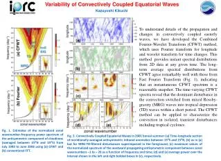
6. Wave-number frequency spectrum of convectively coupled equatorial waves CLAUS Tb Averaged 15ºS-15ºN, 1983–2005 Symmetric component Courtesy of G. Kiladis

7. Wave-number frequency spectrum of convectively coupled equatorial waves 1.25 Days Westward Power Eastward Power 96 Days

8. Wave-number frequency spectrum of convectively coupled equatorial waves Kelvin

9. Wave-number frequency spectrum of convectively coupled equatorial waves Dispersion curves superimposed 90 m 8 m

10. Wave-number frequency spectrum of convectively coupled equatorial waves 25 m

11. Wave-number frequency spectrum of convectively coupled equatorial waves Outgoing Longwave Radiation (OLR) Average: 15ºS-15ºN, 1979–2001 Symmetric component Background removed Wheeler and Kiladis, 1999

12. Kelvin wave over the Indian Ocean

13. Kelvin-domain-filtered symmetric OLR variance Wheeler et al. 2000 All seasons Peak variance at 0o, 90oE. Broad region of variance extending across the IO and into the western PO. KWs events can occur any time of the year.

14. Kelvin-domain-filtered symmetric OLR variance Wheeler et al. 2000 All seasons

15. KWs over the Indian Ocean Wheeler et al. 2000

18. Kelvin wave over the Pacific Ocean

19. Kelvin-domain-filtered total OLR variance May to September

20. Kelvin wave over the Pacific Ocean May to September

21. OLR Lag (days) 14 m s-1

22. OLR (red: increased cloudiness); ECMWF 1000-hPa u, v (vectors), z (contours) Horizontal structure

23. Horizontal structure

24. Observed KWs: Vertical structure, T Straub and Kiladis 2003 Wave Motion Temperature at Majuro (radiosonde, 7N, 171E)

25. Observed KWs: Vertical structure, q Straub and Kiladis 2003 Wave Motion Specific humidity at Majuro (radiosonde, 7N, 171E)

26. Kelvin wave over Central Africa

27. Kelvin-domain-filtered symetric OLR variance in Spring (MAM)

28. Kelvin-domain-filtered symetric OLR variance in Spring (MAM)

29. AA EA IO PO Kelvin-wave-filtered OLR variance 90 50 Wheeler and Kiladis 1999 The Kelvin wave domain is represented by the green polygon 25 12 8 (5oS-5oN) meridional mean Kelvin wave filtered OLR variance • Peaks from the Amazon-Atlantic (AA) in March to the Pacific ocean (PO) in June. • Strongest signal over Equatorial Africa (EA) in April • Role of the surface favoring the Kelvin wave growth. • Equatorial position of the ITCZ in spring.

30. L H Horizontal structure OLR (shading, W/m2)‏ Wind at 850 hPa (vector, m/s)‏ Surface Pressure (contours, Pa) • OLR and dynamical signal centered on the equator along the ITCZ. • Winds are primarily zonal. • Low pressure (convergence) and easterlies to east of lowest OLR • High pressure (divergence) and westerlies to west of lowest OLR

31. Comparison with theoretical structure cat3 Solution of the shallow water model Convection is collocated with the theoretical convergence region

32. 90 50 25 12 8 Characterization in the spectrum Wavelength : 50 ≤  ≤ 90°(longitude) ⇨ Zonal wavenumber : 4 ≤ k ≤ 7 Period of 5-6 days: 8 ≤ c ≤ 18 ms-1 Wheeler and Kiladis 1999

33. Vertical structure OLR (Wm-2) • Lower troposphere: • Moist collocated with the lowest OLR. • Dry is to the west of lowest OLR. • Upper troposphere: moist is to the west of lowest OLR. • progression from shallow to deep convection followed by stratiform clouds. q (g/kg) moist dry Pressure (hPa) T (degK) cold warm • Lower troposphere: • Warm is to the east of lowest OLR. • Cold is to the west of lowest OLR. • Upper troposphere: warm is collocated with lowest OLR.

34. Observed Kelvin wave morphology Straub and Kiladis 2003 Wave Motion

35. Generalized evolution of a convectively coupled equatorial wave Kiladis et al., 2009

36. Interaction with MCSs and diurnal cycle

37. CLAUS Tb 1997 MCSs 20 m/s Kelvin waves 12 m/s

38. Kelvin wave impact on the MCSs • (1984-2002) Composite MCS surface cover, 2 classes (sizes) considered : • The smallest, effective radius < 200 km • The biggest, effective radius > 480 km • no or weak perturbation of the small MCSs by KW • Strong modulation of the big MCSs by the Kelvin wave • Convection is essentially triggered by the orography • Kelvin wave impact mostly on the organization of the MCSs Time (hours) Small MCSs Big MCSs

39. Diurnal cycle of the convection • Brightness temperature • Mar-Apr 1984-2002 • averaged from 5°S-5°N Composite Anomalies Mean diurnal cycle Positive OLR time (hours) Negative OLR • MCSs are triggered near and on the relief • Diurnal cycle marked every day • Enhancement of the convection evident during the wave active phase, especially over the Congo Basin

40. Origin of KWs over South America Courtesy of George Kiladis Liebmann et al., 2009

41. OLR and 200 hPa Flow Regressed against Kelvin-filtered OLR (scaled -20 W m2) at eq, 60W for January-June 1979-2004 Day-4 Streamfunction (contours 5 X 105 m2 s-1) Wind (vectors, largest around 5 ms-1) OLR (shading starts at +/- 6 W s-2), negative blue

42. OLR and 200 hPa Flow Regressed against Kelvin-filtered OLR (scaled -20 W m2) at eq, 60W for January-June 1979-2004 Day-3 Streamfunction (contours 5 X 105 m2 s-1) Wind (vectors, largest around 5 ms-1) OLR (shading starts at +/- 6 W s-2), negative blue

43. OLR and 200 hPa Flow Regressed against Kelvin-filtered OLR (scaled -20 W m2) at eq, 60W for January-June 1979-2004 Day-2 Streamfunction (contours 5 X 105 m2 s-1) Wind (vectors, largest around 5 ms-1) OLR (shading starts at +/- 6 W s-2), negative blue

44. OLR and 200 hPa Flow Regressed against Kelvin-filtered OLR (scaled -20 W m2) at eq, 60W for January-June 1979-2004 Day-1 Streamfunction (contours 5 X 105 m2 s-1) Wind (vectors, largest around 5 ms-1) OLR (shading starts at +/- 6 W s-2), negative blue

45. OLR and 200 hPa Flow Regressed against Kelvin-filtered OLR (scaled -20 W m2) at eq, 60W for January-June 1979-2004 Day 0 Streamfunction (contours 5 X 105 m2 s-1) Wind (vectors, largest around 5 ms-1) OLR (shading starts at +/- 6 W s-2), negative blue

46. OLR and 200 hPa Flow Regressed against Kelvin-filtered OLR (scaled -20 W m2) at eq, 60W for January-June 1979-2004 Day+1 Streamfunction (contours 5 X 105 m2 s-1) Wind (vectors, largest around 5 ms-1) OLR (shading starts at +/- 6 W s-2), negative blue

47. OLR and 200 hPa Flow Regressed against Kelvin-filtered OLR (scaled -20 W m2) at eq, 60W for January-June 1979-2004 Day+2 Streamfunction (contours 5 X 105 m2 s-1) Wind (vectors, largest around 5 ms-1) OLR (shading starts at +/- 6 W s-2), negative blue

48. OLR and 200 hPa Flow Regressed against Kelvin-filtered OLR (scaled -20 W m2) at eq, 60W for January-June 1979-2004 Day+3 Streamfunction (contours 5 X 105 m2 s-1) Wind (vectors, largest around 5 ms-1) OLR (shading starts at +/- 6 W s-2), negative blue

49. The dates are then separated by additional criteria before compositing: Dates are found with a 1.5 standard deviations negative OLR anomalies at 60W, Eq. “Pacific” cases: 3 days before key date Kelvin-filtered OLR more than 16 Wm-2 below mean at 95W, 2.5N “South America” cases: 3 days before key date, 30-day high- pass filtered OLR more than 50 Wm-2 below mean at 60W, 20S. Period: Nov 1979-May 2006 53 Pacific cases 48 South America cases 4 common cases

50. Conclusions for South America • There are at least two mechanisms that force Kelvin waves over South America a) upper levels disturbance propagating along the equator from the Pacific b) lower levels cold surge from southern South America: (e.g., Garreaud and Wallace 1998; Garreaud 2000) • Not all South American (cold) events force Kelvin waves • Some Kelvin waves may be initiated in-situ