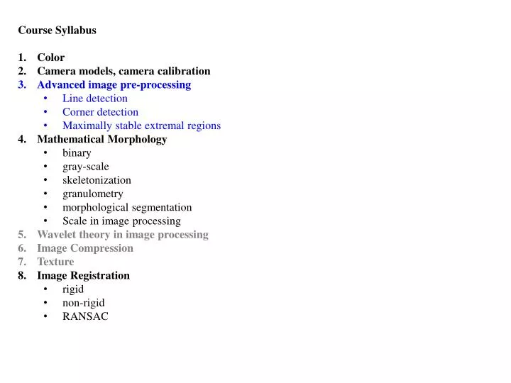
Course Syllabus Color Camera models, camera calibration Advanced image pre-processing

Course Syllabus • Color • Camera models, camera calibration • Advanced image pre-processing • Line detection • Corner detection • Maximally stable extremal regions • Mathematical Morphology • binary • gray-scale • skeletonization • granulometry • morphological segmentation • Scale in image processing • Wavelet theory in image processing • Image Compression • Texture • Image Registration • rigid • non-rigid • RANSAC

References • Book: Chapter 5, Image Processing, Analysis, and Machine Vision, Sonka et al, latest edition (you may collect a copy of the relevant chapters from my office) • Papers: • Harris and Stephens, 4th Alvey Vision Conference, 147-151, 1988. • Matas et al, Image Vision Geometry, 22:761-767, 2004

Topics • Line detection • Interest points • Corner Detection • Moravec detector • Facet model • Harris corner detection • Maximally stable extremal regions

Line detection • Useful in remote sensing, document processing etc. • Edges: • boundaries between regions with relatively distinct gray-levels • the most common type of discontinuity in an image

Line detection • Useful in remote sensing, document processing etc. • Edges: • boundaries between regions with relatively distinct gray-levels • the most common type of discontinuity in an image • Lines: • instances of thin lines in an image occur frequently enough • it is useful to have a separate mechanism for detecting them.

Line detection: How? • Possible approaches: Hough transform

Line detection: How? • Possible approaches: Hough transform (more global analysis and may not be considered as a local pre-processing technique)

Line detection: How? • Possible approaches: Hough transform (more global analysis and may not be considered as a local pre-processing technique) • Convolve with line detection kernels

Line detection: How? • Possible approaches: Hough transform (more global analysis and may not be considered as a local pre-processing technique) • Convolve with line detection kernels • How to detection lines along other directions?

Lines and corner for correspondence • Interest points for solving correspondence problems in time series data. • Corners are better than lines in solving the above

Lines and corner for correspondence • Interest points for solving correspondence problems in time series data. • Corners are better than lines in solving the above • Consider that we want to solve point matching in two images ?

Lines and corner for correspondence • Interest points for solving correspondence problems in time series data. • Corners are better than lines in solving the above • Consider that we want to solve point matching in two images • A vertex or corner provides better correspondence ?

? Corners • Challenges • Gradient computation is less reliable near a corner due to ambiguity of edge orientation

? Corners • Challenges • Gradient computation is less reliable near a corner due to ambiguity of edge orientation • Corner detector are usually not very robust.

? Corners • Challenges • Gradient computation is less reliable near a corner due to ambiguity of edge orientation • Corner detector are usually not very robust. • This deficiency is overcome either by manual intervention or large redundancies.

? Corners • Challenges • Gradient computation is less reliable near a corner due to ambiguity of edge orientation • Corner detector are usually not very robust. • This deficiency is overcome either by manual intervention or large redundancies. • The later approach leads to many more corners than needed to estimate transforms between two images.

Corner detection • Moravec detector: detects corners as the pixels with locally maximal contrast

Corner detection • Moravec detector: detects corners as the pixels with locally maximal contrast • Differential approaches: • Beaudet’s approach: Corners are measured as the determinant of the Hessian. • Note that the determinant of a Hesian is equivalent to the product of the min & max Gaussian curvatures

Continued … • Using a bi-cubic facet model

Harris corner detector • Key idea: Measure changes over a neighborhood due to a shift and then analyze its dependency on shift orientation

Harris corner detector • Key idea: Measure changes over a neighborhood due to a shift and then analyze its dependency on shift orientation • Orientation dependency of the response for lines Δ Δ

Harris corner detector • Key idea: Measure changes over a neighborhood due to a shift and then analyze its dependency on shift orientation • Orientation dependency of the response for lines Δ Δ Δ Δ

Harris corner detector • Key idea: Measure changes over a neighborhood due to a shift and then analyze its dependency on shift orientation • Orientation dependency of the response for lines Δ Δ Δ Δ Δ High response for shifts along the edge direction; low responses for shifts toward orthogonal direction direction Anisotropic response Δ

Key idea: continued … • Orientation dependence of the shift response for corners Δ Δ Δ Δ Δ High response for shifts along all directions Isotropic response Δ

Harris corner: mathematical formulation • An image patch or neighborhood W is shifted by a shift vector Δ = [Δx, Δy]T

Harris corner: mathematical formulation • An image patch or neighborhood W is shifted by a shift vector Δ = [Δx, Δy]T • A corner does not have the aperture problem and therefore should show high shift response for all orientation of Δ.

Harris corner: mathematical formulation • An image patch or neighborhood W is shifted by a shift vector Δ = [Δx, Δy]T • A corner does not have the aperture problem and therefore should show high shift response for all orientation of Δ. • The square intensity difference between the original and the shifted image over the neighborhood W is

Harris corner: mathematical formulation • An image patch or neighborhood W is shifted by a shift vector Δ = [Δx, Δy]T • A corner does not have the aperture problem and therefore should show high shift response for all orientation of Δ. • The square intensity difference between the original and the shifted image over the neighborhood W is • Apply first-order Taylor expansion

Continued …

Harris matrix • The matrix AW is called the Harris matrix and its symmetric and positive semi-definite.

Harris matrix • The matrix AW is called the Harris matrix and its symmetric and positive semi-definite. • Eigen-value decomposition of of AW gives eigenvectors and eigenvalues (λ1, λ2) of the response matrix. • .

Harris matrix • The matrix AW is called the Harris matrix and its symmetric and positive semi-definite. • Eigen-value decomposition of of AW gives eigenvectors and eigenvalues (λ1, λ2) of the response matrix. • Three distinct situations: • Both λ1 and λ2 are small  no edge or corner; a flat region

Harris matrix • The matrix AW is called the Harris matrix and its symmetric and positive semi-definite. • Eigen-value decomposition of of AW gives eigenvectors and eigenvalues (λ1, λ2) of the response matrix. • Three distinct situations: • Both λ1 and λ2 are small  no edge or corner; a flat region • λi is large but λji is small  existence of an edge; no corner

Harris matrix • The matrix AW is called the Harris matrix and its symmetric and positive semi-definite. • Eigen-value decomposition of of AW gives eigenvectors and eigenvalues (λ1, λ2) of the response matrix. • Three distinct situations: • Both λ1 and λ2 are small  no edge or corner; a flat region • λi is large but λji is small  existence of an edge; no corner • Both λ1 and λ2 are large  existence of a corner

Harris matrix • The matrix AW is called the Harris matrix and its symmetric and positive semi-definite. • Eigen-value decomposition of of AW gives eigenvectors and eigenvalues (λ1, λ2) of the response matrix. • Three distinct situations: • Both λ1 and λ2 are small  no edge or corner; a flat region • λi is large but λji is small  existence of an edge; no corner • Both λ1 and λ2 are large  existence of a corner • Avoid eigenvalue decomposition and compute a single response measure • Harris response function • A value of κ between 0.04 and 0.15 has be used in literature.

Algorithm: Harris corner detection • Filter the image with a Gaussian

Algorithm: Harris corner detection • Filter the image with a Gaussian • Estimate intensity gradient in two coordinate directions

Algorithm: Harris corner detection • Filter the image with a Gaussian • Estimate intensity gradient in two coordinate directions • For each pixel c and a neighborhood window W • Calculate the local Harris matrix A

Algorithm: Harris corner detection • Filter the image with a Gaussian • Estimate intensity gradient in two coordinate directions • For each pixel c and a neighborhood window W • Calculate the local Harris matrix A • Compute the response function R(A)

Algorithm: Harris corner detection • Filter the image with a Gaussian • Estimate intensity gradient in two coordinate directions • For each pixel c and a neighborhood window W • Calculate the local Harris matrix A • Compute the response function R(A) • Choose the best candidates for corners by selecting thresholds on the response function R(A)

Course Syllabus Color Camera models, camera calibration Advanced image pre-processing