Download
1 / 51
520 likes | 626 Views
CPU Scheduling. Fan Wu Department of Computer Science and Engineering Shanghai Jiao Tong University Spring 2012. Basic Concepts. Maximize CPU utilization obtained with multiprogramming CPU–I/O Burst Cycle – Process execution consists of a cycle of CPU execution and I/O wait

E N D
CPU Scheduling Fan Wu Department of Computer Science and Engineering Shanghai Jiao Tong University Spring 2012
Basic Concepts • Maximize CPU utilization obtained with multiprogramming • CPU–I/O Burst Cycle – Process execution consists of a cycle of CPU execution and I/O wait • CPU burst distribution
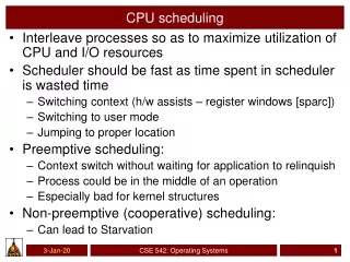
CPU Scheduler • Selects from among the processes in ready queue, and allocates the CPU to one of them • Queue may be ordered in various ways • CPU scheduling decisions may take place when a process: 1. Switches from running to waiting state 2. Switches from running to ready state 3. Switches from waiting to ready • Terminates • Scheduling under 1, 3, and 4 is nonpreemptive, scheduling under 2 is preemptive
Dispatcher • Dispatcher module gives control of the CPU to the process selected by the short-term scheduler; this involves: • switching context • switching to user mode • jumping to the proper location in the user program to restart that program • Dispatch latency – time it takes for the dispatcher to stop one process and start another running
Scheduling Criteria • CPU utilization – keep the CPU as busy as possible • Throughput – # of processes that complete their execution per time unit • Turnaround time – amount of time to execute a particular process. The interval from the time of submission of a process to the time of completion is the turnaround time. • Waiting time – amount of time a process has been waiting in the ready queue • Response time – amount of time it takes from when a request was submitted until the first response is produced, not output (for time-sharing environment)
CPU Scheduling Algorithms • First-Come, First-Served (FCFS) Scheduling • Shortest-Job-First (SJF) Scheduling • Priority Scheduling (PS) • Round-Robin Scheduling (RR) • Multilevel Queue Scheduling • Multilevel Feedback Queue Scheduling
P1 P2 P3 0 24 27 30 First-Come, First-Served (FCFS) Scheduling ProcessCPU BurstArrival Time P1 24 0 P2 3 1 P3 3 2 • The Gantt Chart for the schedule is: • Waiting time for P1 = 0; P2 = 24-1=23; P3 = 27-2=25 Average waiting time: (0 + 23 + 25)/3 = 16 • Turnaround time for P1 = 24; P2 = 27-1=26; P3 = 30-2=28 Average turnaround time: (24 + 26 + 28)/3 = 26
P2 P3 P1 0 3 6 30 FCFS Scheduling (Cont.) Process CPU Burst Arrival Time P1 24 2 P2 3 0 P3 3 1 • The Gantt chart for the schedule is: • Waiting time for P1 = 4;P2 = 0; P3 = 2 • Average waiting time: (4 + 0 + 2)/3 = 2 • Much better than previous case • Convoy effect - short process behind long process • Consider one CPU-bound and many I/O-bound processes
FCFS Scheduling (Cont.) ProcessCPU Burst I/O BurstCPU Burst Arrival Time P1 12 3 12 0 P2 1 2 2 1 P3 1 2 2 2 • The Gantt Chart for the schedule is: • Waiting time for • P1 = 15-12-3=0 • P2 = (12-1)+(27-13-2)=23 • P3 = (13-2)+(29-14-2)=24 • Turnaround time for P1 = 27; P2 = 29-1=28; P3 = 31-2=29 • CPU utilization 30/31 = 96.77% P3 P1 P1 P2 P2 P3 12 13 14 15 27 29 31 0
Shortest-Job-First (SJF) Scheduling • Associate with each process the length of its next CPU burst • Use these lengths to schedule the process with the shortest time • SJF is optimal – gives minimum average waiting time for a given set of processes • The difficulty is knowing the length of the next CPU request • Could ask the user
Determining Length of Next CPU Burst • Can only estimate the length – should be similar to the previous one • Then pick process with shortest predicted next CPU burst • Can be done by using the length of previous CPU bursts, using exponential moving average • Commonly, α is set to ½
Examples of Exponential Averaging • =0 • n+1 = n • Recent history does not count • =1 • n+1 = tn • Only the actual last CPU burst counts • If we expand the formula, we get: n+1 = tn+(1 - ) tn-1+ … +(1 - )j tn-j+ … +(1 - )n +1 0 • Since both and (1 - ) are less than or equal to 1, each successive term has less weight than its predecessor
Example of SJF ProcessArriva l TimeBurst Time P10.0 6 P2 2.0 8 P34.0 7 P45.0 3 • SJF scheduling chart • Average waiting time = (3 + 16 + 9 + 0) / 4 = 7 P3 P2 P4 P1 0 3 9 16 24
P1 P3 P4 P2 P1 0 5 1 10 17 26 Example of Shortest-remaining-time-first • We now add the concepts of varying arrival times and preemption to the analysis ProcessA arri Arrival TimeTBurst Time P10 8 P2 1 4 P32 9 P43 5 • PreemptiveSJF Gantt Chart • Average waiting time = [(10-1)+(1-1)+(17-2)+(5-3)]/4 = 26/4 = 6.5
Priority Scheduling • A priority number (integer) is associated with each process • The CPU is allocated to the process with the highest priority (smallest integer highest priority) • Preemptive • Nonpreemptive • SJF is priority scheduling where priority is the inverse of predicted next CPU burst time • Problem:Starvation – low priority processes may never execute • Solution: Aging – as time progresses increase the priority of the process
P1 P5 P3 P4 P2 0 6 1 16 18 19 Example of Priority Scheduling ProcessA arri Burst TimeTPriority P1 10 3 P2 1 1 P32 4 P41 5 P5 5 2 • Priority scheduling Gantt Chart • Average waiting time = 8.2 msec
Round Robin (RR) • Round Robin (RR) is similar to FCFS scheduling, but preemption is added to switch between processes. • Each process gets a small unit of CPU time (time quantum q), usually 10-100 milliseconds. After this time has elapsed, the process is preempted and added to the end of the ready queue. • If there are n processes in the ready queue and the time quantum is q, then each process gets 1/n of the CPU time in chunks of at most q time units at once. No process waits more than (n-1)q time units before next execution. • Timer interrupts every quantum to schedule next process • Performance • q large FIFO • q small q must be large with respect to context switch, otherwise overhead is too high
P1 P2 P3 P1 P1 P1 P1 P1 0 10 14 18 22 26 30 4 7 Example of RR with Time Quantum = 4 ProcessBurst Time P1 24 P2 3 P3 3 • The Gantt chart is: • Typically, higher average turnaround than SJF, but better response • q should be large compared to context switch time • q usually 10ms to 100ms, context switch < 10 usec • What’s the number of context switch?
Time Quantum and Context Switch Time • Context switching: the process switch not caused by a voluntary yielding of CPU from the running process
Turnaround Time Varies With The Time Quantum 80% of CPU bursts should be shorter than q
Multilevel Queue • Ready queue is partitioned into separate queues, e.g.: • foreground (interactive) • background (batch) • Process permanently in a given queue • Each queue has its own scheduling algorithm: • foreground – RR • background – FCFS • Scheduling must be done between the queues: • Fixed priority scheduling; (i.e., serve all from foreground then from background). Possibility of starvation. • Time slice – each queue gets a certain amount of CPU time which it can schedule amongst its processes; e.g., 80% to foreground in RR, 20% to background in FCFS
Multilevel Feedback Queue • A process can move between the various queues; aging can be implemented this way • Multilevel-feedback-queue scheduler defined by the following parameters: • number of queues • scheduling algorithms for each queue • method used to determine when to upgrade a process • method used to determine when to demote a process • method used to determine which queue a process will enter when that process needs service
Example of Multilevel Feedback Queue Q1 • Three queues: • Q1 – RR with time quantum 8 milliseconds • Q2 – RR with time quantum 16 milliseconds • Q3 – FCFS Q2 Q3
Multilevel Feedback Queue • Scheduling • A new job enters queue Q1which is servedFCFS • When it gains CPU, job receives 8 milliseconds • If it does not finish in 8 milliseconds, job is moved to queue Q2 • At Q2 job is again served FCFS and receives 16 additional milliseconds • If it still does not complete, it is preempted and moved to queue Q3 • If a process does not use up its quantum in the current level, it will keep its current queuing level and be put into the end of the queue. Then, it can still get the same amount of quantum (not remaining quantum) next time when it is picked.
Example of Using Multilevel Feedback Queue ProcessA arri Arrival TimeTBurst Time P10 36 P2 16 20 P320 12 • The Gantt chart is: P1 P1 P2 P3 P1 P2 P3 P1 0 8 16 24 32 48 60 64 68
Thread Scheduling • Distinction between user-level and kernel-level threads • When threads supported, threads scheduled, not processes • Many-to-one and many-to-many models, thread library schedules user-level threads to run on kernel-level threads • Known as process-contention scope (PCS) since scheduling competition is within the process • Typically done via priority set by programmer • Kernel thread scheduled onto available CPU is system-contention scope (SCS)– competition among all threads in system
Pthread Scheduling • API allows specifying either PCS or SCS during thread creation • PTHREAD_SCOPE_PROCESS schedules threads using PCS scheduling • Schedules user-level threads onto available LWPs • Number of LWPs is maintained by the thread library • PTHREAD_SCOPE_SYSTEM schedules threads using SCS scheduling • Creates and binds an LWP for each user-level thread • In fact, implements the one-to-one mapping • Can be limited by OS – Linux and Mac OS X only allow PTHREAD_SCOPE_SYSTEM
Pthread Scheduling API #include <pthread.h> #include <stdio.h> #define NUM_THREADS 5 int main(int argc, char *argv[]) { int i; pthread_t tid[NUM THREADS]; pthread_attr_t attr; /* get the default attributes */ pthread_attr_init(&attr); /* set the scheduling algorithm to PROCESS or SYSTEM */ pthread_attr_setscope(&attr, PTHREAD_SCOPE_SYSTEM); /* create the threads */ for (i = 0; i < NUM_THREADS; i++) pthread_create(&tid[i], &attr, runner,NULL);
Pthread Scheduling API /* now join on each thread */ for (i = 0; i < NUM_THREADS; i++) pthread_join(tid[i], NULL); } /* Each thread will begin control in this function */ void *runner(void *param) { printf("I am a thread\n"); pthread exit(0); }
Multiple-Processor Scheduling • CPU scheduling is more complex when multiple CPUs are available • Homogeneous processors within a multiprocessor • Asymmetric multiprocessing–one processor handles all scheduling decisions, I/O processing, and other system activities; while the other processors just execute user code. • only one processor accesses the system data structures, alleviating the need for data sharing • Symmetric multiprocessing (SMP)– each processor is self-scheduling, all processes in common ready queue, or each has its own private queue of ready processes • Processor affinity – process has affinity for processor on which it is currently running • soft affinity • hard affinity
Multicore Processors • Recent trend to place multiple processor cores on same physical chip • Faster and consumes less power • Multiple threads per core also growing • Takes advantage of memory stall to make progress on another thread while memory retrieve happens
Virtualization and Scheduling • Virtualization software schedules multiple guests onto CPU(s) • Each guest doing its own scheduling • Not knowing it doesn’t own the CPUs • Can result in poor response time • Can effect time-of-day clocks in guests • Can undo good scheduling algorithm efforts of guests
Operating System Examples • Linux scheduling • Solaris scheduling • Windows XP scheduling
Linux Scheduling • Preemptive, priority based • Constant order O(1) scheduling time • Two priority ranges: real-time and time-sharing • Real-time range from 0 to 99 and nice value from 100 to 140 • Map into global priority with numerically lower values indicating higher priority • Higher priority gets larger time quanta • Task run-able as long as time left in time slice (active) • If no time left (expired), not run-able until all other tasks use their slices • All run-able tasks tracked in per-CPU runqueue data structure • Two priority arrays (active, expired) • Tasks indexed by priority • When no more active, arrays are exchanged
Linux Scheduling (Cont.) • Real-time scheduling according to POSIX.1b • Real-time tasks have static priorities • All other tasks dynamic based on nice value plus or minus 5 • Interactivity of task determines plus or minus • More interactive -> more minus • Priority recalculated when task expired • This exchanging arrays implements adjusted priorities
Solaris • Priority-based scheduling • Six classes available • Time sharing (default) • Interactive • Real time • System • Fair Share • Fixed priority • Given thread can be in one class at a time • Each class has its own scheduling algorithm • Time sharing is multi-level feedback queue • Loadable table configurable by sysadmin
Solaris Scheduling (Cont.) • Scheduler converts class-specific priorities into a per-thread global priority • Thread with highest priority runs next • Runs until (1) blocks, (2) uses time slice, (3) preempted by higher-priority thread • Multiple threads at same priority selected via RR
Windows Scheduling • Windows uses priority-based preemptive scheduling • Highest-priority thread runs next • Dispatcher is scheduler • Thread runs until (1) blocks, (2) uses time slice, (3) preempted by higher-priority thread • Real-time threads can preempt non-real-time • 32-level priority scheme • Variable class is 1-15, real-time class is16-31 • Priority 0 is memory-management thread • Queue for each priority • If no run-able thread, runs idle thread
Windows Priority Classes • Win32 API identifies several priority classes to which a process can belong • REALTIME_PRIORITY_CLASS, HIGH_PRIORITY_CLASS, ABOVE_NORMAL_PRIORITY_CLASS,NORMAL_PRIORITY_CLASS, BELOW_NORMAL_PRIORITY_CLASS, IDLE_PRIORITY_CLASS • All are variable except REALTIME • A thread within a given priority class has a relative priority • TIME_CRITICAL, HIGHEST, ABOVE_NORMAL, NORMAL, BELOW_NORMAL, LOWEST, IDLE • Priority class and relative priority combine to give numeric priority • Base priority is NORMAL within the class • If quantum expires, priority lowered, but never below base • If wait occurs, priority boosted depending on what was waited for • Foreground window given 3x priority boost
Pop Quiz • Draw Gantt charts to illustrate the execution of the processes using the following scheduling algorithm: (1) FCFS, (2) nonpreemptive SJF, (3) preemptive SJF, (4) nonpreemptive priority, (5) preemptive priority, and (6) RR with time quantum=2 • Calculate the average turnaround time when using each of the above scheduling algorithms • Count the number of context switches when using each of the above scheduling algorithms