Boosting, dimension reduction and a preview of the return to Big Data

1. Boosting, dimension reduction and a preview of the return to Big Data Peter Fox Data Analytics – ITWS-4963/ITWS-6965 Week 13a, April 22, 2014

2. Reading • http://data-informed.com/focus-predictive-analytics/

3. Weak models … • A weak learner: a classifier which is only slightly correlated with the true classification (it can label examples better than random guessing) • A strong learner: a classifier that is arbitrarily well-correlated with the true classification. • Can a set of weak learners create a single strong learner?

4. Boosting • … reducing bias in supervised learning • most boosting algorithms consist of iteratively learning weak classifiers with respect to a distribution and adding them to a final strong classifier. • typically weighted in some way that is usually related to the weak learners' accuracy. • After a weak learner is added, the data is reweighted: examples that are misclassified gain weight and examples that are classified correctly lose weight • Thus, future weak learners focus more on the examples that previous weak learners misclassified.

5. Diamonds require(ggplot2) # or load package first data(diamonds) head(diamonds) # look at the data! # ggplot(diamonds, aes(clarity, fill=cut)) + geom_bar() ggplot(diamonds, aes(clarity)) + geom_bar() + facet_wrap(~ cut) ggplot(diamonds) + geom_histogram(aes(x=price)) + geom_vline(xintercept=12000) ggplot(diamonds, aes(clarity)) + geom_freqpoly(aes(group = cut, colour = cut))

7. Using diamonds… boost (glm) > mglmboost<-glmboost(as.factor(Expensive) ~ ., data=diamonds,family=Binomial(link="logit")) > summary(mglmboost) Generalized Linear Models Fitted via Gradient Boosting Call: glmboost.formula(formula = as.factor(Expensive) ~ ., data = diamonds, family = Binomial(link = "logit")) Negative Binomial Likelihood Loss function: { f <- pmin(abs(f), 36) * sign(f) p <- exp(f)/(exp(f) + exp(-f)) y <- (y + 1)/2 -y * log(p) - (1 - y) * log(1 - p) }

8. Using diamonds… boost (glm) > summary(mglmboost) #continued Number of boosting iterations: mstop = 100 Step size: 0.1 Offset: -1.339537 Coefficients: NOTE: Coefficients from a Binomial model are half the size of coefficients from a model fitted via glm(... , family = 'binomial'). See Warning section in ?coef.mboost (Intercept) carat clarity.L -1.5156330 1.5388715 0.1823241 attr(,"offset") [1] -1.339537 Selection frequencies: carat (Intercept) clarity.L 0.50 0.42 0.08

10. bodyfat • The response variable is the body fat measured by DXA (DEXfat), which can be seen as the gold standard to measure body fat. • However, DXA measurements are too expensive and complicated for a broad use. • Anthropometric measurements as waist or hip circumferences are in comparison very easy to measure in a standard screening. • A prediction formula only based on these measures could therefore be a valuable alternative with high clinical relevance for daily usage.

12. bodyfat ## regular linear model using three variables lm1 <- lm(DEXfat ~ hipcirc + kneebreadth + anthro3a, data = bodyfat) ## Estimate same model by glmboost glm1 <- glmboost(DEXfat ~ hipcirc + kneebreadth + anthro3a, data = bodyfat) # We consider all available variables as potential predictors. glm2 <- glmboost(DEXfat ~ ., data = bodyfat) # or one could essentially call: preds <- names(bodyfat[, names(bodyfat) != "DEXfat"]) ## names of predictors fm <- as.formula(paste("DEXfat ~", paste(preds, collapse = "+"))) ## build formula

13. Compare linear models > coef(lm1) (Intercept) hipcirckneebreadth anthro3a -75.2347840 0.5115264 1.9019904 8.9096375 > coef(glm1, off2int=TRUE) ## off2int adds the offset to the intercept (Intercept) hipcirckneebreadth anthro3a -75.2073365 0.5114861 1.9005386 8.9071301 Conclusion?

14. > fm DEXfat ~ age + waistcirc + hipcirc + elbowbreadth + kneebreadth + anthro3a + anthro3b + anthro3c + anthro4 > coef(glm2, which = "") ## select all. (Intercept) age waistcirchipcircelbowbreadthkneebreadth anthro3a anthro3b anthro3c -98.8166077 0.0136017 0.1897156 0.3516258 -0.3841399 1.7365888 3.3268603 3.6565240 0.5953626 anthro4 0.0000000 attr(,"offset") [1] 30.78282

15. plot(glm2, off2int = TRUE)

16. plot(glm2, ylim = range(coef(glm2, which = preds)))

17. > summary(bodyfat) age DEXfatwaistcirchipcircelbowbreadthkneebreadthanthro3a Min. :19.00 Min. :11.21 Min. : 65.00 Min. : 88.00 Min. :5.200 Min. : 7.200 Min. :2.400 1st Qu.:42.00 1st Qu.:22.32 1st Qu.: 78.50 1st Qu.: 96.75 1st Qu.:6.200 1st Qu.: 8.600 1st Qu.:3.540 Median :56.00 Median :29.63 Median : 85.00 Median :103.00 Median :6.500 Median : 9.200 Median :3.970 Mean :50.86 Mean :30.78 Mean : 87.38 Mean :105.28 Mean :6.508 Mean : 9.301 Mean :3.869 3rd Qu.:62.00 3rd Qu.:39.33 3rd Qu.: 99.75 3rd Qu.:111.15 3rd Qu.:6.900 3rd Qu.: 9.800 3rd Qu.:4.155 Max. :67.00 Max. :62.02 Max. :117.00 Max. :132.00 Max. :7.400 Max. :11.800 Max. :4.680 anthro3b anthro3c anthro4 Min. :2.580 Min. :2.050 Min. :3.180 1st Qu.:4.060 1st Qu.:3.480 1st Qu.:5.040 Median :4.390 Median :3.990 Median :5.530 Mean :4.291 Mean :3.886 Mean :5.398 3rd Qu.:4.660 3rd Qu.:4.345 3rd Qu.:5.840 Max. :5.010 Max. :4.620 Max. :6.370

18. Other forms of boosting • Gamboost = Generalized Additive Model - Gradient boosting for optimizing arbitrary loss functions, where component-wise smoothing procedures are utilized as (univariate) base-learners.

19. > gam1 <- gamboost(DEXfat ~ bbs(hipcirc) + bbs(kneebreadth) + bbs(anthro3a),data = bodyfat) > #Using plot() on a gamboost object delivers automatically the partial effects of the different base-learners: > par(mfrow = c(1,3)) ## 3 plots in one device > plot(gam1) ## get the partial effects # bbs, bols, btree..

21. > gam2 <- gamboost(DEXfat ~ ., baselearner = "bbs", data = bodyfat,control = boost_control(trace = TRUE)) [ 1] .................................................. -- risk: 515.5713 [ 53] .............................................. Final risk: 460.343 > set.seed(123) ## set seed to make results reproducible > cvm <- cvrisk(gam2) ## default method is 25-fold bootstrap cross-validation

22. > cvm Cross-validated Squared Error (Regression) gamboost(formula = DEXfat ~ ., data = bodyfat, baselearner = "bbs", control = boost_control(trace = TRUE)) 1 2 3 4 5 6 7 8 9 10 109.44043 93.90510 80.59096 69.60200 60.13397 52.59479 46.11235 40.80175 36.32637 32.66942 11 12 13 14 15 16 17 18 19 20 29.66258 27.07809 24.99304 23.11263 21.55970 20.40313 19.16541 18.31613 17.59806 16.96801 21 22 23 24 25 26 27 28 29 30 16.48827 16.07595 15.75689 15.47100 15.21898 15.06787 14.96986 14.86724 14.80542 14.74726 31 32 33 34 35 36 37 38 39 40 14.68165 14.68648 14.64315 14.67862 14.68193 14.68394 14.75454 14.80268 14.81760 14.87570 41 42 43 44 45 46 47 48 49 50 14.90511 14.92398 15.00389 15.03604 15.07639 15.10671 15.15364 15.20770 15.23825 15.30189 51 52 53 54 55 56 57 58 59 60 15.31950 15.35630 15.41134 15.46079 15.49545 15.53137 15.57602 15.61894 15.66218 15.71172 61 62 63 64 65 66 67 68 69 70 15.72119 15.75424 15.80828 15.84097 15.89077 15.90547 15.93003 15.95715 15.99073 16.03679 71 72 73 74 75 76 77 78 79 80 16.06174 16.10615 16.12734 16.15830 16.18715 16.22298 16.27167 16.27686 16.30944 16.33804 81 82 83 84 85 86 87 88 89 90 16.36836 16.39441 16.41587 16.43615 16.44862 16.48259 16.51989 16.52985 16.54723 16.58531 91 92 93 94 95 96 97 98 99 100 16.61028 16.61020 16.62380 16.64316 16.64343 16.68386 16.69995 16.73360 16.74944 16.75756 Optimal number of boosting iterations: 33

23. > mstop(cvm) ## extract the optimal mstop [1] 33 > gam2[ mstop(cvm) ] ## set the model automatically to the optimal mstop Model-based Boosting Call: gamboost(formula = DEXfat ~ ., data = bodyfat, baselearner = "bbs", control = boost_control(trace = TRUE)) Squared Error (Regression) Loss function: (y - f)^2 Number of boosting iterations: mstop = 33 Step size: 0.1 Offset: 30.78282 Number of baselearners: 9

24. plot(cvm)

25. > names(coef(gam2)) ## displays the selected base-learners at iteration 30 [1] "bbs(waistcirc, df = dfbase)" "bbs(hipcirc, df = dfbase)" "bbs(kneebreadth, df = dfbase)" [4] "bbs(anthro3a, df = dfbase)" "bbs(anthro3b, df = dfbase)" "bbs(anthro3c, df = dfbase)" [7] "bbs(anthro4, df = dfbase)" > gam2[1000, return = FALSE] # return = FALSE just supresses "print(gam2)" [ 101] .................................................. -- risk: 423.9261 [ 153] .................................................. -- risk: 397.4189 [ 205] .................................................. -- risk: 377.0872 [ 257] .................................................. -- risk: 360.7946 [ 309] .................................................. -- risk: 347.4504 [ 361] .................................................. -- risk: 336.1172 [ 413] .................................................. -- risk: 326.277 [ 465] .................................................. -- risk: 317.6053 [ 517] .................................................. -- risk: 309.9062 [ 569] .................................................. -- risk: 302.9771 [ 621] .................................................. -- risk: 296.717 [ 673] .................................................. -- risk: 290.9664 [ 725] .................................................. -- risk: 285.683 [ 777] .................................................. -- risk: 280.8266 [ 829] .................................................. -- risk: 276.3009 [ 881] .................................................. -- risk: 272.0859 [ 933] .................................................. -- risk: 268.1369 [ 985] .............. Final risk: 266.9768

26. > names(coef(gam2)) ## displays the selected base-learners, now at iteration 1000 [1] "bbs(age, df = dfbase)" "bbs(waistcirc, df = dfbase)" "bbs(hipcirc, df = dfbase)" [4] "bbs(elbowbreadth, df = dfbase)" "bbs(kneebreadth, df = dfbase)" "bbs(anthro3a, df = dfbase)" [7] "bbs(anthro3b, df = dfbase)" "bbs(anthro3c, df = dfbase)" "bbs(anthro4, df = dfbase)” > glm3 <- glmboost(DEXfat ~ hipcirc + kneebreadth + anthro3a, data = bodyfat,family = QuantReg(tau = 0.5), control = boost_control(mstop = 500)) > coef(glm3, off2int = TRUE) (Intercept) hipcirckneebreadthanthro3a -63.5164304 0.5331394 0.7699975 7.8350858

28. Compare to rpart > fattree<-rpart(DEXfat ~ ., data=bodyfat) > plot(fattree) > text(fattree) > labels(fattree) [1] "root" "waistcirc< 88.4" "anthro3c< 3.42" "anthro3c>=3.42" "hipcirc< 101.3" "hipcirc>=101.3" [7] "waistcirc>=88.4" "hipcirc< 109.9" "hipcirc>=109.9"

30. cars

31. iris

32. cars

34. Optimizing Coefficients: (Intercept) speed -60.331204 3.918359 attr(,"offset") [1] 42.98 Call: glmboost.formula(formula = dist ~ speed, data = cars, control = boost_control(mstop = 1000), family = Laplace()) Coefficients: (Intercept) speed -47.631025 3.402015 attr(,"offset") [1] 35.99999

36. Sparse matrix example > coef(mod, which = which(beta > 0)) V306 V1052 V1090 V3501 V4808 V5473 V7929 V8333 V8799 V9191 2.1657532 0.0000000 4.8756163 4.7068006 0.4429911 5.4029763 3.6435648 0.0000000 3.7843504 0.4038770 attr(,"offset") [1] 2.90198

38. Aside: Boosting and SVM… • Remember “margins” from the SVM? Partitioning the “linear” or transformed space? • In boosting we are effectively (not explicitly) attempting to maximize the minimum margin of any training example

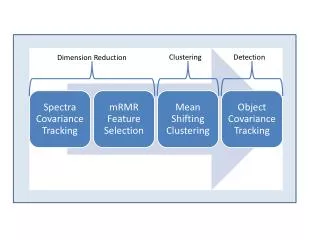
39. Dimension reduction.. • Principle component analysis (PCA) and metaPCA (in R) • Singular Value Decomposition • Feature selection, reduction • Clustering • Why? • Curse of dimensionality – or – some subset of the data should not be used as it adds noise • What is it? • Various methods to reach an optimal subset

40. Feature selection • The goodness of a feature/feature subset is dependent on measures • Various measures • Information measures • Distance measures • Dependence measures • Consistency measures • Accuracy measures

41. Libraries in R that you used… • MetaPCA (prcomp, metaPCA) • EDR (effective dimension reduction) • dr

42. Lab 6

43. prostate data (lab 7).

44. Demo (lab 8) library(EDR) # effective dimension reduction ###install.packages("edrGraphicalTools") ###library(edrGraphicalTools) demo(edr_ex1) demo(edr_ex2) demo(edr_ex3) demo(edr_ex4)

45. Lab 9 library(dr) data(ais) # default fitting method is "sir" s0 <- dr(LBM~log(SSF)+log(Wt)+log(Hg)+log(Ht)+log(WCC)+log(RCC)+ log(Hc)+log(Ferr),data=ais) # Refit, using a different function for slicing to agree with arc. summary(s1 <- update(s0,slice.function=dr.slices.arc)) # Refit again, using save, with 10 slices; the default is max(8,ncol+3) summary(s2<-update(s1,nslices=10,method="save")) # Refit, using phdres. Tests are different for phd, and not # Fit using phdres; output is similar for phdy, but tests are not justifiable. summary(s3<- update(s1,method="phdres")) # fit using ire: summary(s4 <- update(s1,method="ire")) # fit using Sex as a grouping variable. s5 <- update(s4,group=~Sex)

46. > s0 dr(formula = LBM ~ log(SSF) + log(Wt) + log(Hg) + log(Ht) + log(WCC) + log(RCC) + log(Hc) + log(Ferr), data = ais) Estimated Basis Vectors for Central Subspace: Dir1 Dir2 Dir3 Dir4 log(SSF) 0.150963358 -0.0501785457 0.10898336 -0.002210206 log(Wt) -0.916480522 -0.1942298625 -0.20123696 -0.089722026 log(Hg) -0.131538894 0.6854750758 0.71997546 -0.663097774 log(Ht) -0.093358860 -0.0433408964 0.46445398 0.290838658 log(WCC) 0.004467838 0.0001833808 0.04497590 0.071904557 log(RCC) -0.188973540 0.3475652934 0.29496908 0.037056363 log(Hc) 0.274758965 -0.6058301419 -0.34196615 0.678877114 log(Ferr) -0.005631238 0.0130588502 -0.08702709 0.015547214 Eigenvalues: [1] 0.95766163 0.24504161 0.10707594 0.09041305

47. > summary(s1 <- update(s0,slice.function=dr.slices.arc)) Call: dr(formula = LBM ~ log(SSF) + log(Wt) + log(Hg) + log(Ht) + log(WCC) + log(RCC) + log(Hc) + log(Ferr), data = ais, slice.function = dr.slices.arc) Method: sir with 11 slices, n = 202. Slice Sizes: 19 19 19 19 19 19 19 18 18 18 15 Estimated Basis Vectors for Central Subspace: Dir1 Dir2 Dir3 Dir4 log(SSF) 0.143177 -0.0476079 -0.02815 0.003785 log(Wt) -0.879504 -0.1425841 0.23303 -0.094970 log(Hg) -0.195963 0.6318503 0.24483 -0.509424 log(Ht) -0.058923 -0.1100757 -0.87893 0.217803 log(WCC) -0.007276 -0.0029772 -0.05309 0.043056 log(RCC) -0.167736 0.3924936 -0.19711 -0.213689 log(Hc) 0.368652 -0.6418658 -0.26373 0.796849 log(Ferr) -0.002697 0.0002593 0.03492 0.039116 Dir1 Dir2 Dir3 Dir4 Eigenvalues 0.9572 0.2275 0.09368 0.07319 R^2(OLS|dr) 0.9980 0.9981 0.99839 0.99864 Large-sample Marginal Dimension Tests: Stat dfp.value 0D vs >= 1D 284.78 80 0.00000 1D vs >= 2D 91.43 63 0.01113 2D vs >= 3D 45.48 48 0.57690 3D vs >= 4D 26.55 35 0.84694

48. > summary(s2<-update(s1,nslices=10,method="save")) Call: dr(formula = LBM ~ log(SSF) + log(Wt) + log(Hg) + log(Ht) + log(WCC) + log(RCC) + log(Hc) + log(Ferr), data = ais, slice.function = dr.slices.arc, nslices = 10, method = "save") Method: save with 10 slices, n = 202. Slice Sizes: 21 21 20 20 20 25 24 22 20 9 Estimated Basis Vectors for Central Subspace: Dir1 Dir2 Dir3 Dir4 log(SSF) 0.127709 -0.00907 0.01018 -0.06144 log(Wt) -0.905004 -0.07107 -0.15734 0.25774 log(Hg) -0.056187 0.50674 -0.34064 -0.38087 log(Ht) 0.399868 0.36613 0.68439 -0.54216 log(WCC) 0.032608 0.02733 0.02277 0.03474 log(RCC) -0.008463 0.15137 -0.24136 -0.47219 log(Hc) -0.021630 -0.76164 0.57591 0.51526 log(Ferr) 0.002116 -0.01670 0.01631 -0.03360 Dir1 Dir2 Dir3 Dir4 Eigenvalues 0.9389 0.6611 0.5129 0.4653 R^2(OLS|dr) 0.9936 0.9950 0.9985 0.9989 Large-sample Marginal Dimension Tests: Stat df(Nor) p.value(Nor) p.value(Gen) 0D vs >= 1D 378.3 324 0.02012 0.1071 1D vs >= 2D 279.6 252 0.11214 0.3116 2D vs >= 3D 179.9 189 0.67101 0.5160 3D vs >= 4D 134.3 135 0.50176 0.2786

49. S0 v. S2

50. S3 and S4