Abstract

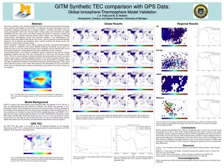
1. Abstract Since the ionosphere is the interface between the Earth and space environments and impacts radio, television and satellite communication, it is imperative to model and predict it well. The ionosphere undergoes changes due to plasma transport, chemistry and impact ionization during geomagnetic storms and intervals where energy, mass and momentum are rapidly transferred from the solar wind to the Earth’s space environment. Ionospheric changes can cause scintillation in Global Positioning System (GPS) signals, and interruption in satellite communication. Geomagnetic storms also generate changes in the plasmasphere and therefore impact the radiation belts and the ring current. Unless ionospheric and plasmaspheric dynamics can be detected and predicted, space weather problems will impact society with regards to communication and space travel. At the University of Michigan, Aaron Ridley created the Global Ionosphere-Thermosphere Model (GITM) to contribute to the Space Weather Modeling Framework, whose goal is to model from Sun to the mud. GITM covers the main ionospheric electron density peak, but not the topside ionosphere or plasmasphere (which also contributes to electron density). A good determination of an effective ionospheric model is looking at how well the electron distribution matches with data. One way of doing this is to look at the total electron content (TEC). TEC is the column density of electrons between two points within an area of one meter squared, which gives an altitude integrated measure of the electron density variation. Fig. 1 shows a TEC extraction from GITM during quiet time. In this study GITM is compared to GPS TEC data to determine the effects of the topside ionosphere and plasmasphere on TEC values and to test the accuracy of the model. Note however, that observations of TEC are limited to where there are ground based receivers and therefore most areas of the Earth (oceans) are not sampled. Global Results Regional Results US Europe Japan Malaysia Fig 6: A closer look at the regions with distinction in the global view or with the most GPS receivers and each regions average difference between GPS TEC and GITM TEC over a year from October 2007 to September 2008. GITM Synthetic TEC comparison with GPS Data:Global Ionosphere-Thermosphere Model ValidationJ. A. Feldt and M. B. Moldwin Atmospheric, Oceanic, and Space Sciences, University of Michigan Fig. 1: A GITM Global TEC observation where the color indicates the magnitude of TEC. Note that the highest values of TEC are at noon local time and near the equator. Model Background GITM is a model of the thermosphere and ionosphere within the altitudes of 90 to 500 km. It uses an altitude-based grid that stretches in latitude and altitude and assumes a non-hydrostatic solution, which strengthens the model in the auroral regions. GITM is initialized by the densities and temperatures from the bottom of the atmosphere, data from MSIS and IRI, or from a previous run. It allows for input from IRI, MSIS, satellite data (such as CHAMP), F10.7 data from the Flare Irradiance Spectral Model from LASP, NOAA/POES Hemispheric Power Index Data, and IMF data. GITM also allows the user to turn on, off or set values for various source terms. For this study all source terms were left on or set to the default values and the model was initiated from the densities and temperatures at the bottom of the atmosphere. Fig 3: These twelve plots show a whole year of differences between GPS Tec and GITM synthetic TEC. Note that the dark blue indicates GITM over estimating TEC. Also note that through the months of October to May the Malaysian difference displays a distinct underestimation. GPS TEC The GPS TEC data used in this study is from the Madrigal Database at the Haystack Observatory at MIT. TEC is measured by the delayed phase of radio transmission from GPS satellites, which transmit in dual frequencies. Conclusions GITM is greatly overestimating TEC, which is unexpected since it covers only a portion of the atmosphere and it has a much lower density profile than IRI, which is known to be highly comparable to data. Looking at individual regions, GITM overestimates more in the Summer to Fall months over US and Europe, while remaining fairly constant in Japan. Malaysia shows a much greater difference in the beginning of the year, which may be due to the biases of the GPS receivers in Malaysia. Next step would be to turn on and off source terms in GITM’s code and also to check the biases of GPS receivers in Malaysia to determine what is causing these great differences. Resources Coster, A., and A. Komjathy (2008), Space Weather and the Global Positioning System, Space Weather, 6, 15-19. Ridley, A.J., Y. Deng, and G. Tóth (2006), The global ionosphere-thermosphere model, J. of Atmo. and Solar-Terr. Phys., 68, 839-864. Jee, G., Schunk, R.W., and Scherliess, L. (2005), Comparison of IRI-2001 with TOPEX TEC measurements, Journal of Atmospheric and Solar-Terrestrial Physics, 67, 365–380 Acknowledgements Feldt is supported by the NASA Graduate Student Research Project through JPL and the Rackham Merit Fellowship. Fig 4: A comparison of the density profiles of IRI and GITM on 01/03/08 at 12 UT. Fig 5: A comparison of the global average difference between GPS TEC and GITM TEC over a year from October 2007 to September 2008. Fig. 2: A Madrigal World Wide GPS Receiver Network observation where the color indicates the magnitude of TEC. Note that, just like the GITM observation the highest values of TEC are at noon local time and near the equator.