Download
1 / 38
390 likes | 555 Views
I nventory planning and control. Source: Corbis. QUANTITY DISCOUNTS. Is the price reductions for large orders, offered to customers to induce them to buy in large quantities. The price per box decreases as the order quantity increases. Quantity Discount.

E N D
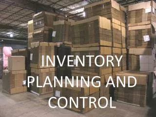
Inventoryplanning and control Source: Corbis
QUANTITY DISCOUNTS • Is the price reductions for large orders, offered to customers to induce them to buy in large quantities.
Quantity Discount • If the quantity discount are offered, the buyer must weigh the potential benefits of reduced purchase price and the few orders that will result from buying in large quantities against the increase in carrying costs caused by higher average inventories.
QD Assumptions • Only one item is involved • Annual demand is known • The usage rate is constant • Usage occurs continually but production occurs periodically • The production rate is constant • Lead time does not vary
Buyers goal’s with QD • Is to select the order quantity that will minimize total costs, where total costs is the sum of carrying cost, ordering costs and purchasing costs.
TC = (Carrying + ordering + purchase) cost (Q/2)H + (D/Q)S + PD Where P = Unit price
Remember in the basic EOQ model, determination of order size does not involve the purchasing costs. The price per unit is the same for all order sizes
Objective of QD Model • Is to identify an order quantity that will represent the lowest total cost for the entire set of curves • There are two general cases of the model
1. When CC are constant • Compute the common minimum point • Only one of the unit prices will have the minimum point in its feasible range since the range do not overlap, identify that range; • If the feasible minimum pint is on the lowest price range, that is the optimal order quantity
When CC are constant Cont… • If the feasible minimum point is in any range, compute the total cost for the minimum and for the price breaks of all lowest unit costs. • Compare the total cost; the quantity (minimum point or price break) that yields the lowest total cost is the optimal order quantity
Worked example 1. The maintenance department of a large hospital uses about 816 cases of liquid cleanser annually. Ordering cost are $12, carrying cost are $4 per case a year and the new price schedule indicate orders of less than 50 cases will cost $20 per case, 50 to 79 cases will cost $18 per case, 80 to 99 cases will cost $17 per case and larger order will cost $16 per case. Determine the optimal order quantity and the total cost.
2. When CC are expressed as a % of price • Beginning with the lowest unit price, compute the minimum points for each price range until you find a feasible minimum point (i.e. until a minimum point falls in the quantity range for its price)
CC are expressed as a % Cont… • If the minimum point for the lowest unit price is feasible, it is the optimal order quantity. • If the minimum point is not feasible in the lowest price range, compare the total cost at the price break for the lowest prices with the total cost of the largest feasible minimum point. • The quantity that yields the lowest total cost is the optimal
Worked example 2. Surge electric uses 4,000 toggle switches a year. Switches are priced as follows; 1 to 499,90 cents each, 500 to 999, 85 cents each and 1000 or more, 80 cents each. It costs approximatelly $30 to prepare an order and receive it, and carrying cost are 40% of purchase price per unit on an annual basis. Determine the optimal order quantity and the total annual cost.
EPQ Cont… • Gradual replacement; Other names are: • The economic batch quantity (EBQ) • The Economic manufactory quantity (EMQ) • EPQ, the replenishment occurs over a time period rather than in one lot
EPQ Cont… • A typical example of this is where an internal order is placed for a batch of parts to be produced on a machine. • Thus, the size of the inventory will increase (P). After the batch has been completed the machine will be reset and demand will continue to deplete the inventory level (D) until production of the next batch begins.
EPQ Cont… • Thus; during the production phase of the cycle, inventory builds up at a rate equal to the difference between production and usage rates. • e.g. If the daily production rate is 20 units and the daily usage rates is 5units, inventory will build up at the rate of 20 - 5 equal to 15 units per day.
EPQ Cont… • As long as production occurs, the inventory level will continue to build; when production ceases, the inventory level will begin to decrease. • Hence, the inventory level will be maximum at the point where production ceases. • When the amount of inventory on hand is exhausted, production is resumed and the cycle repeats itself.
EPQ Cont… • Because the company makes the product itself, there are no ordering costs as such, • Nonetheless, with every production run (batch) there are set up costs (the costs required to prepare the equipment for the job i.e. clearing, adjusting , changing tools and fixtures).
EPQ Cont… • The larger the run size, the few the number of runs needed and, hence, the lower the annual set-up cost • The number of runs or bathes is D/Q • The annual set-up cost is equal to the number of runs per year times the set-up cost per run (D/Q) S
EPQ Cont… • Therefore TC min = carrying cost + set-up costs (I max/2) H + (D/Q) S Where Imax = Maximum Inventory • The maximum inventory level Imax = Q/p (p – u)
EPQ Cont… • The cycle time (the time between orders or between the beginnings of runs) for the economic run size model is a function of the run size and usage (demand) rate. Cycle time = Q/u
EPQ Cont… • Similarly, the run time (the production phase of the cycle) a function of the run size and the production rate: Run time = Q/p
EPQ Cont… • Average inventory level is; I average = Imax/2
Production quantity Q Noninstantaneous Replenishment On-hand inventory Time
Production quantity Q Noninstantaneous Replenishment Demand during production interval On-hand inventory p – d Time
Production quantity Q Demand during production interval On-hand inventory p – d Time Noinstantaneous Replenishment
Production quantity Q Demand during production interval On-hand inventory p – d Time Production and demand Demand only TBO Noinstantaneous Replenishment
Production quantity Q Demand during production interval On-hand inventory p – d Time Production and demand Demand only TBO Noinstantaneous Replenishment
Production quantity Q Demand during production interval Imax On-hand inventory Maximum inventory p – d Time Production and demand Demand only TBO Special Inventory Models
Production quantity Q Demand during production interval Imax On-hand inventory Maximum inventory Imax = (p – d) = Q( ) p – d p Q p p – d Time Production and demand Demand only TBO Noinstantaneous Replenishment
Production quantity Q Demand during production interval Imax On-hand inventory Maximum inventory Imax 2 D Q C = (H) + (S) p – d Time Production and demand Demand only TBO Noinstantaneous Replenishment
Production quantity Q Demand during production interval Imax On-hand inventory Maximum inventory C = ( ) + (S) Q p – d 2 p D Q p – d Time Production and demand Demand only TBO Noinstantaneous Replenishment
Production quantity Q Demand during production interval Imax On-hand inventory Maximum inventory p p – d 2DS H ELS = p – d Time Production and demand Demand only TBO Noinstantaneous Replenishment
Worked example 3. • A toy manufacturer uses 48,000 rubber wheels per year for its popular dump truck series. The firm makes its own wheels, which it can produce at a rate of 800 per day. The toy trucks are assembled uniformly over the entire year. Carrying cost is $ 1 per wheel a year. Setup cost for a production run of wheels is $ 45. The firm operates 240 days per year. Determine the:
Example 3. Cont… (a) optimal run size (b) minimum total annual cost for carrying and setup (c) Cycle time for the optimal run size (d) Run size