Download
1 / 9
100 likes | 378 Views
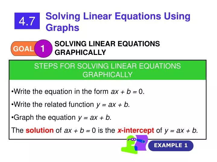
Solving Linear Equations Using Graphs. 4.7. SOLVING LINEAR EQUATIONS GRAPHICALLY. 1. GOAL. EXAMPLE 1. Write the equation in the form ax + b = 0. Write the related function y = ax + b. Graph the equation y = ax + b. The solution of ax + b = 0 is the x -intercept of y = ax + b.

E N D
Solving Linear Equations Using Graphs 4.7 SOLVING LINEAR EQUATIONS GRAPHICALLY 1 GOAL EXAMPLE 1 • Write the equation in the form ax + b = 0. • Write the related function y = ax + b. • Graph the equation y = ax + b. • The solution of ax + b = 0 is the x-intercept of y = ax + b. STEPS FOR SOLVING LINEAR EQUATIONS GRAPHICALLY
y x (0, –3) EXAMPLE 2 Extra Example 1 Solve –x – 3 = 0.5x algebraically. Check graphically. Solve –x – 3 = 0.5x for x: x = –2 The x-intercept is –2, which confirms the solution. To check graphically: Rewrite as ax + b = 0: –1.5x – 3 = 0 Write the related function: y = –1.5x – 3 Graph the equation: b = –3 m = –1.5 =
y x Extra Example 2 To solve graphically: Rewrite as ax + b = 0: Write the related function: Graph the equation: (0, –1) The solution is the x-intercept: The solution can be checked algebraically by solving the original equation. Note: The same solution will be found even if you rewrite the equation as 2x + 1 = 0.
Solving Linear Equations Using Graphs 4.7 2 APPROXIMATING SOLUTIONS IN REAL LIFE GOAL EXAMPLE 4
Extra Example 4 Based on census data from 1987 to 1995, a model for the hourly wage w of people employed in the production of computers and related goods in the United States is w = 0.409t + 10.74, where t is the number of years since 1987. According to this model, in what year will the hourly wage for these workers be approximately $18.10? To solve, graph the equation and find the value of t when the value of w = 18.10.
w 20 18 16 14 12 10 t 0 4 8 10 12 14 16 18 20 EXAMPLE 5 Extra Example 4 w = 0.409t + 10.74 When w = 18.10, t ≈ 18, which corresponds to the year 2005.
w 20 18 16 14 12 10 t 0 4 8 10 12 14 16 18 20 Extra Example 5 Write and graph a function for each side of the equation 18.10 = 0.409t + 10.74 from Extra Example 4. What is the t-coordinate of the point where the two graphs intersect? Graph w = 18.10. Graph w = 0.409t + 10.74 The t coordinate of the point of intersection is 18.
Checkpoint The average speeds in miles per hour of the first six winners (1911–1916) of the Indianapolis 500 can be modeled by the equation y = 1.84x + 80, where x is the number of years since 1911 and y is the average speed in miles per hour. Use this model to find the average speed of Ralph DePalma, the 1915 winner. Regardless of the way you choose to solve this problem, the solution is 87.36 miles per hour.
QUESTION: What linear function is related to the equation 4x + 3 = 5? ANSWER: y = 4x – 2