Download
1 / 7
70 likes | 176 Views
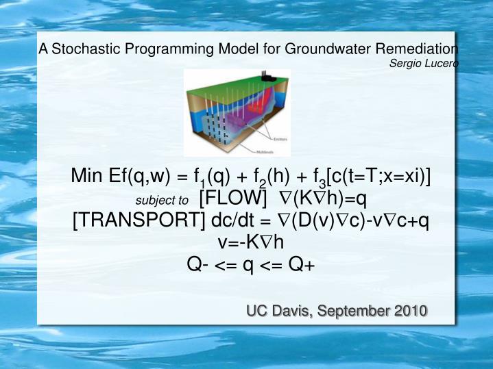
Min Ef(q,w) = f 1 (q) + f 2 (h) + f 3 [c(t=T;x=xi)] subject to [FLOW] (K h)=q [TRANSPORT] dc/dt = (D(v) c)-v c+q v=-K h Q- <= q <= Q+. A Stochastic Programming Model for Groundwater Remediation Sergio Lucero. UC Davis, September 2010. Elements of the Model.

E N D
Min Ef(q,w) = f1(q) + f2(h) + f3[c(t=T;x=xi)] subject to [FLOW] (Kh)=q [TRANSPORT] dc/dt = (D(v)c)-vc+q v=-Kh Q- <= q <= Q+ A Stochastic Programming Model for Groundwater RemediationSergio Lucero UC Davis, September 2010
Elements of the Model • Min f(q)=E{d'q + l||h||2 + Sj[c(t=T;x=xi)-c*]} • Q pumping rates, h hydraulic heads, c*: acceptable pollution level • 2 convex cost terms, easy to compute ((Kh)=q) • 1 non-convex term requiring a PDE solution dc/dt = (D(v)c)-vc+q • Python < MATLAB << C implementation < RWHET • Stochasticity given by uncertain soil parameters (eg:porosity) • Nonlinearity stems from D(v) = aI + bvv' • Decision Flow: q→h→v→D→c→f
2D test case • Estimate numerical complexity • Pumping wells close to four corners • Observe anisotropy, diffusion,dispersion • See whether PHA converges! • Scenario problems: Min d'q+l||h||2+Perf[c(t=T)]+Wk'q+r||q-q||2 • Optimality validation: test Ef(q*+ez)
Kernel Solutions of the Flow Eqn • Observe that nwells << nnodes • So every time we (approx) solve (Kh)=q, only very little changes in the RHS!! • Solution: PRESOLVE and reuse! • [i=0] AKhBC=qBC [i=1...nwells] AKhi=ei • q=Sqiei => h=hBC+Sqihi • Replaces an O(nxd) linear system by matvec!
Python Implementation • Straightforward with numpy+scipy
Costly (4D) loops!! • At least this part must be coded in C(types) • Modularity of code allows for Random Walk
Results • PHA converges without monotonicity • Importance of rho choice • Scenario solutions can be suboptimal • Local optimality is validated a posteriori • Nx=100 solved in under an hour (1CPU) • Parallelization on Amazon's EC2+Starcluster • Should allow to solve 3D, Nx=1000, 32 scen