Download
1 / 27
270 likes | 366 Views
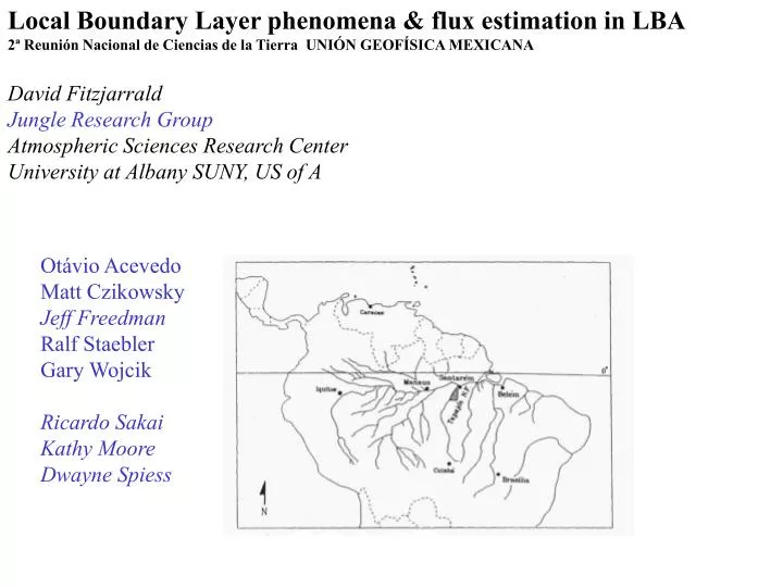
Local Boundary Layer phenomena & flux estimation in LBA 2ª Reunión Nacional de Ciencias de la Tierra UNIÓN GEOFÍSICA MEXICANA David Fitzjarrald Jungle Research Group Atmospheric Sciences Research Center University at Albany SUNY, US of A. Otávio Acevedo Matt Czikowsky Jeff Freedman

E N D
Local Boundary Layer phenomena & flux estimation in LBA 2ª Reunión Nacional de Ciencias de la Tierra UNIÓN GEOFÍSICA MEXICANA David Fitzjarrald Jungle Research Group Atmospheric Sciences Research Center University at Albany SUNY, US of A Otávio Acevedo Matt Czikowsky Jeff Freedman Ralf Staebler Gary Wojcik Ricardo Sakai Kathy Moore Dwayne Spiess
Precipitation in central Amazon is highly seasonal(from Mendes, MS thesis UFPa, 1999) But the rainfall at the riverside climate stations is biased. (Garstang & Fitzjarrald, 1999, p. 290) Rainfall between 4/16 & 5/14/87, ABLE 2b. Rio Solimões
C flux observations will always be biased by local circulations. Which is more important--”LULC” or river effects? Confluence of the Tapajos & Amazonas rivers near Santarém.
It is nowhere flat, especially at night. Topography in the LBA-Ecology region near Santarém. Weather station & flux tower sites indicated.
It is nowhere homogeneous. Surface type categories in the FLONA Tapajos River is at left.
It is always awkward to do field work at “remote” sites. LBA-Ecology Pasture Site (km 77) Tower Solar panels
“Humble” but continuous, long-term data should be highly prized. (But remember that information goes both ways between modelers & observers.) Automatic weather stations near Belterra (top) and at Fazenda Caboco, km 117 (bottom). JRG, ASRC
With enough data, you can select for the periods for which any budget methods might be most applicable. (Isolated case studies may lead only to anecdotal information.) On light wind days, the river breeze leads to WD reversal.
“Hodographs” made by hour (local time) are useful, if you can wait to get a large enough data set.
IR GOES Visible GOES image (recorded at USP)
1999 LBA-Ecology JRG & USP Average low cloud frequency for May 1999. with the station network, we get areal distribution of incident radiation. Looks like “subtle” topography can be important in the humid tropics.
Recovery from synoptic Disturbance--fair weather Clouds drive the system to A preferred LCL (or RH).
AIRSHEDS!. Drainage outflows seen from “ripples” on a calm morning. (Maryland, US of A) Land Water Synthetic Aperture Radar image of Chesapeake Bay drainage flows. (Winstead et al., 1997).
Lots of things go on inside the rain forest canopy. Vertical profiles at Ducke (Fitzjarrald et al., 1988)
Something completely different. Prototype of the in-canopy sounding system, improving on the G. Parker (right) design. T, q, [CO2]
Observing very local scale advective effects may not be possible if there are no regular local flows to provide a periodic signal. Test observations done by JRG at Harvard Forest (Staebler et al., 2000). Which way is uphill?
Utility of SODAR observations. It doesn’t measure quite what we want. HF, DRAINO (Staebler, JRG). At Harvard Forest... Effects of the local hill extend well into the SBL. (SODAR results and mysteries!)
What we need to do: • Use data compositing creatively. • Deploy remote sensing instruments to get the BL winds (e.g. profilers and acoustic sounders) and concentrations (e.g. DIAL) in horizontal arrays. Operate these networks for several seasons continuously. • Develop hybrid schemes using continuous time series from surface data. Select data for transient periods of weak turbulence and estimate surface flux from ∂C/∂t; use bounding value (envelope) analyses for guidance; take advantage of the early evening, morning transitions. • Do not ignore the role of clouds. Their presence drives the BL toward constant relative humidity equilibrium. Also, cloud base gives an estimate of CBL thickness--can use ceilometer. • Exploit the nocturnal case.(!) Use the regularity of local winds to find the advection terms. Such “natural” boxes as an alpine valleys provide predictable circulations ideal for making composites. Drainage flows from coastal areas carry respiratory CO2 from airsheds over water. Measuring the volume of the outflow and its excess [CO2] allows an independent estimate of the forest respiration rate.