Tree Based Methods for Analyzing Tissue Microarray Data

1. Tree Based Methodsfor Analyzing Tissue Microarray Data Steve Horvath Human Genetics and Biostatistics University of California, Los Angeles

2. Acknowledgements • Horvath Lab • Yunda Huang • Xueli Liu Ph.D. • Zeke Fang Ph.D. • Tuyen Hoang • UCLA Tissue Microarray Core • David Seligson • Aarno Palotie • Clinicians • Hyung Kim • Arie Belldegrun

3. Contents • Statistical issues with tissue microarray (TMA) data • Random forest (RF) predictors • RF clustering • Application of RF clustering to TMA data • Supervised Learning Methods

4. Background TMA data

5. Description of TMA data • TMA data are a high-throughput tool in validating newly-identified biomarker in genome wide discovery • Basic technique was summarized in Kononen et al. 1998

6. Tissue Microarray (TMA) Technology Kononen et al. Nature Medicine 1998 • Hundreds of tiny (typically 0.6 mm diameter) cylindrical tissue cores • densely and precisely arrayed into a single histologic paraffin block. • From this new array block, up to 300 serial 4-8 m thick sections may be produced. • Targets for fluorescence in situ hybridization (FISH) and protein expression by immunohistochemical studies. donor block array block slide

7. Non-normal and highly correlated

8. Several Spots per Pathology CaseSeveral “Scores” per Spot • Each case is usually represented by 4 or more spots • >3 malignant lesions, 1 matched normal • Maximum intensity = Max (1 – 4) • Percent of cells staining = Pos (0 – 100) • Percent of cells staining with the • maximum intensity = PosMax (0 – 100) • Spots have a spot grade: NL,1,2,.. • Indicator of informativeness

9. Histogram of tumor marker expression scores: POS and MAX Percent of Cells Staining(POS) EpCam P53 CA9 Maximum Intensity (MAX)

10. P53 and Ki67: Max versus Pos

11. Characteristics of TMA data • Non-normal, discrete, strongly correlated • Mixed variable types • Pooling (combining) spot measurements across every patient • between 1 to 10 spots of different grade • current strategy pools tumor spots and forms median, mean, minimum or max • Message: tumor marker intensity is measured by up to 12 highly correlated staining scores multicollinearity

12. Our main tool are random forest predictors • Unsupervised analysis of TMA data • RF clustering • Supervised Analysis • RF based pre-validation method

13. Background random forest predictorsL. Breiman 1999

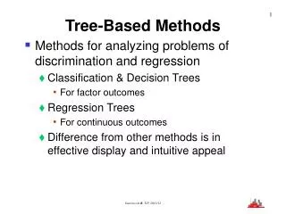
14. Random Forests (RFs) • RFs are a collection of tree predictors such that each tree depends on the values of an independently sampled random vector

15. Classification and Regression Trees (CART) by • Leo Breiman, UC Berkeley • Jerry Friedman, Stanford University • Charles J. Stone, UC Berkeley • Richard Olshen, Stanford University

16. An example of CART • Goal: For the patients admitted into ER, to predict who is at higher risk of heart attack • Training data set: • # of subjects = 215 • Outcome variable = High/Low Risk determined • 19 noninvasive clinical and lab variables were used as the predictors

17. CART construction High 17% Low 83% Is BP <= 91? No Yes High 70% Low 30% High 12% Low 88% Classified as high risk! Is age <= 62.5? No Yes High 2% Low 98% High 23% Low 77% Classified as low risk! Is ST present? Yes No High 50% Low 50% High 11% Low 89% Classified as low risk! Classified as high risk!

18. CART Construction BINARY RECURSIVE PARTITIONING • Binary: split parent node into two child nodes • Recursive: each child node can be treated as parent node • Partitioning: data set is partitioned into mutually exclusive subsets in each split

19. RF Construction …

20. Prediction by plurality voting • The forest consists of N trees. • Class prediction: • Each tree votes for a class; the predicted class C for an observation is the plurality, maxCk [fk(x,T) == C] • Regression random forest: • predicted value is the average prediction

21. Clustering with random forest predictors

22. Intrinsic Proximity Measure • Terminal tree nodes contain few observations • If case i and case j both land in the same terminal node, increase the proximity between i and j by 1. • At the end of the run divide by 2* no. of trees. • Dissimilarity=sqrt(1-Proximity)

23. Casting an unsupervised problem into a supervised RF problem • Key Idea (Breiman 1999) • Label observed data as class 1 • Generate synthetic observations and label them as class 2 • Construct a RF predictor to distinguish class 1 from class 2 • Use the resulting dissimilarity measure in unsupervised analysis

24. How to generate synthetic observations • Synthetic observations are simulated to contain no clusters • e.g. randomly sampling from the product of empirical marginal distributions of the input.

25. RF clustering • Compute distance matrix from RF • distance matrix = sqrt(1-proximity matrix) • Compute the first 2~3 classical multi-dimensional scaling coordinates based on the distance matrix • Conduct partitioning around medoid (PAM) clustering analysis • input parameter=no. of clusters k • use the Euclidean distance between the resulting scaling points

26. Theoretical Study of RF Clustering Ref: Using random forest proximity for unsupervised learning, BIOKDD-CBGI'03, 7th Joint Conference on Information Sciences, Cary, North Carolina.

27. Applying Random Forest Clustering to Tissue Microarray Data--Application to Kidney Cancer Tao Shi and Steve Horvath

28. Scientific Question:Can one discover cancer subtypes based on the protein expression patterns of tumor markers?

29. Why use RF clustering for TMA data? • no need to transform the often highly skewed features • based on ranks of features • natural way of weighing tumor marker contributions to the dissimilarity • elegant way to deal with missing covariates • intrinsic proximity matrix handles mixed variable types well

30. Kidney Multi-marker Data • 366 patients with Renal Cell Carcinoma (RCC) admitted to UCLA between 1989 and 2000. • Immuno-histological measures of total 8 tumor markers were obtained from tissue microarrays constructed from the tumor samples of these patients.

31. MDS plot of clear cell patients • Labeled and colored • by their RF cluster

32. Interpreting the clusters in terms of survival

33. Hierarchical clustering with Euclidean distance leads to less satisfactory results * RF clustering grouping in red

34. RF distance Euclidean distance Euclidean vs. RF Distance

35. Molecular grouping vs. Pathological grouping Molecular Grouping Pathological Grouping 1.0 1.0 0.8 0.8 p = 9.03e-05 0.6 0.6 p = 0.0229 Survival Survival 0.4 0.4 327 patients in cluster 1 and 2 0.2 0.2 316 non-clear cell patients 39 patients in cluster 3 50 clear cell patients 0.0 0.0 0 2 4 6 8 10 12 0 2 4 6 8 10 12 Time to death (years) Time to death (years) Message: molecular grouping is superior to pathological grouping

36. Identify “irregular” patients 1.0 0.8 0.6 Survival 0.4 p = 0.00522 0.2 50 non-clear cell patients Message: molecular grouping can be used to refine clear cell definition. 9 irregular clear cell patients 307 regular clear cell patients 0.0 0 2 4 6 8 10 12 Time to death (years)

37. Detect novel cancer subtypes • Group clear cell grade 2 patients into two clusters with significantly different survival. K-M curves 1.0 0.8 0.6 Survival p value= 0.0125 0.4 0.2 0.0 0 2 4 6 8 10 12 Time to death (years)

38. Results TMA clustering • Clusters reproduce well known clinical subgroups • Ex: global expression differences between clear cell and non-clear cell patients • RF clustering works better than clustering based on the Euclidean distance for TMA data • RF clustering allows one to identify “outlying” tumor samples. • Can detect previously unknown sub-groups

39. Boxplots of tumor marker expression vs. cluster Message: clusters can be explained in terms of tumor expression values, i..e in terms of biological pathways.

40. Conclusions • There is a need to develop tailor made data mining methods for TMA data • Major differences: • highly non-normal data • Euclidean distance metrics seems to be sub-optimal for TMA data • tree or forest based methods work well for kidney and prostate TMA data