Download
1 / 27
270 likes | 390 Views
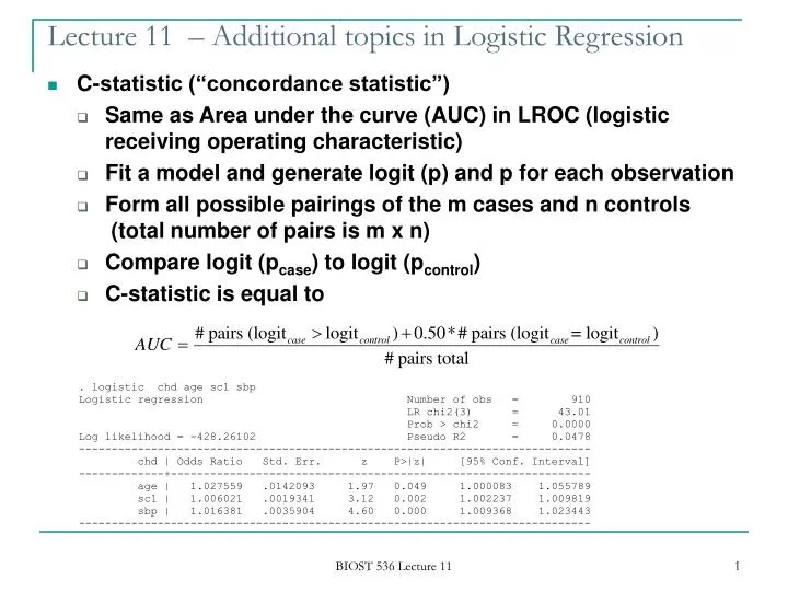
Lecture 11 – Additional topics in Logistic Regression. C-statistic (“concordance statistic”) Same as Area under the curve (AUC) in LROC (logistic receiving operating characteristic) Fit a model and generate logit (p) and p for each observation

E N D
Lecture 11 – Additional topics in Logistic Regression • C-statistic (“concordance statistic”) • Same as Area under the curve (AUC) in LROC (logistic receiving operating characteristic) • Fit a model and generate logit (p) and p for each observation • Form all possible pairings of the m cases and n controls (total number of pairs is m x n) • Compare logit (pcase) to logit (pcontrol) • C-statistic is equal to BIOST 536 Lecture 11
Create all possible pairs of cases (m=178) x number of controls (n=732) = 130,296 • Assess number of pairs where the case logit > control logit • No ties – get the same result as lroc • Can also compute the c-statistic for the validation sample to test prediction in a new sample BIOST 536 Lecture 11
Small sample sizes • Logistic regression LR tests, odds ratio estimates, confidence intervals depend on asymptotic large-sample results • May not work well for small samples • May not even be able to get estimates in some cases if a category has all cases or all controls • Sir DR Cox proposed some small sample exact logistic regression methods in his 1970 text Analysis of Binary Data • Not computationally feasible until an algorithm developed by Hirji, Mehta, and Patel (1987) reduced computations (programs marketed as StatXact and LogXact) • Exact logistic regression uses the sufficient statistics for all covariates in the model: • Condition on the sufficient statistics and consider all permutations of the data consistent with the sufficient statistics • Can derive estimates and confidence intervals BIOST 536 Lecture 11
Small sample sizes • Computation can be extensive • Can stratify by variables that we control for • Methods now included in SAS and Stata (Version 10 on?) • Small dose escalation example • Too small for ordinary logistic regression BIOST 536 Lecture 11
Small sample sizes • Do this example in Stata using exact logistic regression (exlogistic command) • Do an incorrect standard logistic regression first • Wald test and LR disagree BIOST 536 Lecture 11
Small sample sizes • Exact logistic regression does show a significant relationship of deaths with dose and gives odds ratio and permutation-based confidence intervals • Note sufficient statistic is BIOST 536 Lecture 11
Small sample sizes – Example 2 • Two binary covariates • Only 3 outcomes observed • First consider Fisher’s exact test to relate A to outcome • Set up the data using frequency counts BIOST 536 Lecture 11
Small sample sizes – Example 2 • Same answer with exact logistic regression • Now consider both covariates together BIOST 536 Lecture 11
Small sample sizes – Example 3 • Crossover design • Same individuals get tested in all treatments • Outcome is recorded after each treatment • Treatment effect is assumed to wash out quickly after outcome is measured • Order of treatments may still matter • Example has 15 individuals undergoing three treatments but in different orders BIOST 536 Lecture 11
Small sample sizes – Example 3 • Drug: 0 Placebo; 1 Drug A; 2 Drug B • Treat time and drug as categorical variables • Need to group observations within individual (all comparisons are within individual) BIOST 536 Lecture 11
Small sample sizes – Example 3 • Drug A is significantly different than Placebo • Drug B has higher odds ratio than Placebo, but is not statistically significant • Time effects are not strong • Have accounted for the correlation within individual by grouping • Conditioning methods used extensively later BIOST 536 Lecture 11
More on confounding • Confounder is a covariate that is related to the outcome as well as the primary risk factor or scientific variable of interest • “Confounding is the distortion of a disease/exposure association brought about by the association of other factors with both disease and exposure, the latter association with disease being causal” Breslow & Day (1980) • “If any factor either increasing or decreasing the risk of disease besides the characteristic or exposure under study is unequally distributed in the groups that are being compared with regard to the disease, this itself will give rise to differences in disease frequency in the compared groups. Such distortion, termed confounding, leads to an invalid comparison” Lilienfeld & Stolley (1994) BIOST 536 Lecture 11
More on confounding • Criteria for a confounding factor (Rothman & Greenland, 1998) • Confounding factor must be a risk factor for the disease • Confounding factor must be associated with the exposure under study in the source population (the population at risk from which the cases are derived) • Confounding factor must not be affected by exposure or the disease. In particular, it cannot be an intermediate step in the causal path between the exposure and the disease • Choosing confounders for statistical adjustment • Choice should be based on a priori considerations • Study design/protocol specifies particular exposure x disease association under investigation • Confounders selected/measured based on their role as known risk factors for disease BIOST 536 Lecture 11
More on confounding • Best not to select based on internal study results • Selecting on the basis of statistical significance with outcome can leave residual confounding • Selecting on change in association of exposure and outcome may not lead to correct inference • Reporting results • Give unadjusted estimates • Give estimates adjusted for known primary risk factors • Give estimates adjusted for primary and secondary risk factors • How do we adjust? BIOST 536 Lecture 11
Paradigms for controlling for confounding • Experimental methods • Hold all other relevant factors constant • Randomly allocate subjects to treatments • Statistical approaches for controlling for confounding • Estimate conditional treatment effects holding values of confounders constant • Assume constant effect measure within strata – confounders are not effect modifiers • Indirect standardization • Mantel-Haenszel summary odds ratio in stratified analyses • Get adjusted estimates using logistic regression • Traditional method of adjusting for confounding involves comparison of unadjusted versus adjusted estimates • Sometimes called “summarized effect measure” (Newman, 2001) BIOST 536 Lecture 11
Paradigms for controlling for confounding • Estimate marginal treatment effects under simulated randomization • Randomization assumes equal distribution of potential confounders among treatment (exposure) groups • Treatment effects measured by contrasting marginal distributions of response • Direct standardization of rates or proportions • Simulates randomized experiment by fixing the distribution of the confounder to be equal across treatment groups • Compares marginal measures of response between “fixed” treatment groups • Less dependent on modeling assumptions, but less stable statistically and less generalizable to other populations with different confounder distributions BIOST 536 Lecture 11
Paradigms for controlling for confounding • “Causal” analysis of unobserved (“counterfactual”) responses that would have been observed if subjects had been assigned to another treatment • Treatment/exposure effects measured by contrasting marginal distributions of responses (both observed and counterfactual) between treatment groups • Confounding controlled by use of inverse probability weighting of observed responses to compensate for missing counterfactual responses • Example: Probability that treated response is observed is equal to the probability of treatment estimated by logistic regression of treatment category on confounders (“propensity score”) • Assumption of no unmeasured confounders equivalent to assuming that unobserved (counterfactual) responses are “missing at random” in sense of Little and Rubin (1987) BIOST 536 Lecture 11
Direct standardization • Compare response rates under different scenarios where both treatments are applied to equivalent populations assumed to equal the distribution of • Treatment 1 group • Treatment 2 group • 50% Treatment 1 and 50% Treatment 2 • Some other arbitrary population • Difference depends on how population is standardized • Answers “What would be the difference if …” BIOST 536 Lecture 11
Causal models for binary outcome data • Assume that everyone has two possible binary outcomes, Y1 if they received treatment (or were exposed) and Y0 if not treated (or not exposed) • May be written as followsto emphasize that these are the outcomes that would occur if assigned to treatment or not • Counterfactual nature of Y occurs because only one of Y1 and Y0 can be observed • Define R to the the random variable that indicates whether a subject receives treatment (R=1) or not (R=0) • R=1 indicates a subject was selected for treatment • R and the counterfactual Y may be statistically correlated • Observed binary outcome is BIOST 536 Lecture 11
Causal models for binary outcome data • Fundamental problem of causal inference is that difference in expected outcome of treating everyone versus treating no one (LHS) does not equal difference in expected outcomes among those actually treated versus not treated due to bias in allocation of treatment to subjects • Confounding is present if there is not equality between the LHS and RHS of expression (1) • If we randomized, then R and the counterfactual Y are independent, and the LHS may be estimated directly and there is no confounding • Without randomization, we cannot be sure if confounding is present or not BIOST 536 Lecture 11
Causal models for binary outcome data • May be willing to assume that R is independent of the counterfactual Y within strata formed by Z, a composite of measured confounders, i.e. R and Y are conditionally independent given Z • This is an assumption and not verifiable from the data • May be a good assumption if randomization was carried out within strata • If the assumption of conditional independence is true given Z BIOST 536 Lecture 11
Causal models for binary outcome data • Numerator of probability is a standard logistic regression model for outcome given observed treatment and covariates • Denominator is the probability of receiving that treatment given the covariates • Suggest we can estimate these probabilities by using inverse probability weighting (IPW), estimating selection for treatment within strata • IPW results in a synthetic or pseudo-population where treatment (exposure) and the confounders are uncorrelated • Marginal (or crude) measures of treatment effect within the pseudo-population constitutes the causal effect of interest • Direct standardization of effect measure is conceptually and algebraically identical to this marginal causal effect BIOST 536 Lecture 11
Example (Robins, Hernan, & Brumback, 2000) BIOST 536 Lecture 11
Example (Robins, Hernan, & Brumback, 2000) BIOST 536 Lecture 11
Example (Robins, Hernan, & Brumback, 2000) • Note that R and Z are unassociated and that the pseudo-population is twice the size of the original sample • Marginal risk difference is which equals the risk differencefound by direct standardization to a population that has the same fractions in each stratum as the original sample pooled over treatment (or exposure) • Marginal (causal) odds ratio BIOST 536 Lecture 11
Example (Robins, Hernan, & Brumback, 2000) • Crude risk difference is • Crude odds ratio • Note standard errors not shown for the IPW weighted results • Stata can weight inversely by “sampling probabilities” using pweight • Causal modeling is an area of research interest currently BIOST 536 Lecture 11
Propensity scores • Causal inference requires no association between treatment (exposure) and counterfactual outcome Y conditional on Z • What if Z is multidimensional with continuous components, can we find a function of Z such that conditioning on Z, will suffice to meet this independence condition? • Answer: The propensity score can satisfy this independence (Rosenbaum & Rubin, 1983) • Find a model for exposure given covariate vector Z • Stratify or match on estimated propensity score • Estimated association of exposure and disease is a summary over propensity score strata and not necessarily equal to the causal effect • Fine matching may be difficult but crude matching or modeling using the propensity score may allow residual confounding BIOST 536 Lecture 11