Download
1 / 89
890 likes | 1.04k Views
Examples of One-Dimensional Systolic Arrays. Motivation & Introduction. We need a high-performance , special-purpose computer system to meet specific application. I/O and computation imbalance is a notable problem. The concept of Systolic architecture can map high-level

E N D
Motivation & Introduction • We need a high-performance , special-purpose computer • system to meet specific application. • I/O and computation imbalance is a notable problem. • The concept of Systolic architecture can map high-level • computation into hardware structures. • Systolic system works like an automobile assembly line. • Systolic system is easy to implement because of its • regularity and easy to reconfigure. • Systolic architecture can result in cost-effective , high- • performance special-purpose systems for a wide range • of problems.
Pipelined Computations P1 P2 P3 P4 P5 f, e, d, c, b, a • Pipelined program divided into a series of tasks that have to be completed one after the other. • Each task executed by a separate pipeline stage • Data streamedfrom stage to stageto form computation
Pipelined Computations P5 P4 P3 P2 P1 a b c d e f a b c d e f a b c d e f P1 P2 P3 P4 P5 f, e, d, c, b, a a b c d e f a b c d e f time • Computation consists of data streaming through pipeline stages • Execution Time = Time to fill pipeline (P-1) + Time to run in steady state (N-P+1) + Time to empty pipeline (P-1) P = # of processors N = # of data items (assume P < N) This slide must be explained in all detail. It is very important
Pipelined Example: Sieve of Eratosthenes • Goal is to take a list of integers greater than 1 and produce a list of primes • E.g. For input 2 3 4 5 6 7 8 9 10, output is 2 3 5 7 • A pipelined approach: • Processor P_i divides each input by the i-th prime • If the input is divisible (and not equal to the divisor), it is marked (with a negative sign) and forwarded • If the input is not divisible, it is forwarded • Last processor only forwards unmarked (positive) data [primes]
Sieve of Eratosthenes Pseudo-Code Code for processor Pi (and prime p_i): x=recv(data,P_(i-1)) If (x>0) then If (p_i divides x and p_i = x ) then send(-x,P_(i+1) If (p_i does not divide x or p_i = x) then send(x, P_(i+1)) Else Send(x,P_(i+1)) Code for last processor x=recv(data,P_(i-1)) If x>0 then send(x,OUTPUT) P2 P3 P5 P7 out / Processor P_i divides each input by the i-th prime
Programming Issues P13 P17 P2 P3 P5 P7 P11 • Algorithm will take N+P-1 to run where N is the number of data items and P is the number of processors. • Can also consider just the odd bnys or do some initial part separately • In given implementation, number of processors must store all primes which will appear in sequence • Not a scalable approach • Can fix this by having each processor do the job of multiple primes, i.e. mapping logical “processors” in the pipeline to each physical processor • What is the impact of this on performance? processor does the job of three primes
Processors for such operation • In pipelined algorithm, flow of data moves through processors in lockstep. • The design attempts to balance the work so that there is no bottleneck at any processor • In mid-80’s, processors were developed to support in hardware this kind of parallel pipelined computation • Two commercial products from Intel: • Warp (1D array) • iWarp (components for 2D array) • Warp and iWarp were meant to operate synchronously Wavefront Array Processor (S.Y. Kung) was meant to operate asynchronously, • i.e. arrival of data would signal that it was time to execute
Systolic Arrays from Intel • Warp and iWarp were examples of systolic arrays • Systolic means regular and rhythmic, • data was supposed to move through pipelined computational units in a regular and rhythmic fashion • Systolic arrays meant to be special-purpose processors or co-processors. • They were very fine-grained • Processors implement a limited and very simple computation, usually called cells • Communication is very fast, granularity meant to be around one operation/communication!
Systolic Algorithms • Systolic arrays were built to support systolic algorithms, a hot area of research in the early 80’s • Systolic algorithms used pipelining through various kinds of arrays to accomplish computational goals: • Some of the data streaming and applications were very creative and quite complex • CMU a hotbed of systolic algorithm and array research (especially H.T. Kung and his group)
Example 1: “pipelined” polynomial evaluation • Polynomial Evaluation is done by using a Linear array with 2D. • Expression: Y = ((((anx+an-1)*x+an-2)*x+an-3)*x……a1)*x + a0 • Function of PEs in pairs • 1. Multiply input by x • 2. Pass result to right. • 3. Add aj to result from left. • 4. Pass result to right.
Example 1: polynomial evaluation Y = ((((anx+an-1)*x+an-2)*x+an-3)*x……a1)*x + a0 Multiplying processor X is broadcasted • Using systolic array for polynomial evaluation. • This pipelined array can produce a polynomial on new X value on every cycle - after 2n stages. • Another variant: you can also calculate various polynomials on the same X. • This is an example of a deeply pipelined computation- • The pipeline has 2n stages. Adding processor x an-1 an-2 an x x a0 x ………. X + X + X + X +
Example 2:Matrix Vector Multiplication • There are many ways to solve a matrix problems using systolic arrays, some of the methods are: • Triangular Array performing gaussian elimination with neighbor pivoting. • Triangular Array performing orthogonal triangularization. • Simple matrix multiplication methods are shown in next slides.
Example 2:Matrix Vector Multiplication • Matrix Vector Multiplication: • Each cell’s function is: • 1. To multiply the top and bottom inputs. • 2. Add the left input to the product just obtained. • 3. Output the final result to the right. • Each cell consists of an adder and a few registers. • At time t0 the array receives 1, a, p, q, and r ( The other inputs are all zero). • At time t1, the array receive m, d, b, p, q, and r ….e.t.c • The results emerge after 5 steps.
Matrix Multiplication Example 2:Matrix Vector Multiplication - -i - h f g ec d b - a - - n m l PE1 PE2 PE3 z y x q r p • At time t0 the array receives 1, a, p, q, and r ( The other inputs are all zero). • At time t1, the array receive m, d, b, p, q, and r ….e.t.c • The results emerge after 5 steps.
- -i - h f g ec d b - a - - n m l z y x PE1 PE2 PE3 q r p • Each cell (P1, P2, P3) does just one instruction • Multiply the top and bottom inputs, add the left input to the product just obtained, output the final result to the right • The cells are simple • Just an adder and a few registers • The cleverness comes in the order in which you feed input into the systolic array • At time t0, the array receives l, a, p, q, and r • (the other inputs are all zero) • At time t1, the array receives m, d, b, p, q, and r • And so on. • Results emerge after 5 steps To visualize how it works it is good to do a snapshot animation
Systolic Processors, versus Cellular Automata versus Regular Networks of Automata Data Path Block Data Path Block Data Path Block Data Path Block Systolic processor Control Block Control Block Control Block Control Block These slides are for one-dimensional only Cellular Automaton
Systolic Processors, versus Cellular Automata versus Regular Networks of Automata Control Block Control Block Control Block Control Block General and Soldiers, Symmetric Function Evaluator Cellular Automaton Control Block Control Block Control Block Control Block Data Path Block Data Path Block Data Path Block Data Path Block Regular Network of Automata
FIR-filter like structure a4 0 0 0 b2 b1 b4 b3 + + + a4*b4
a3 a4 0 0 b2 b1 b4 b3 + + + a4*b4 a3*b4+a4b3
a2 a3 a4 0 b2 b1 b4 b3 + + + a4*b4 a3*b4+a4b3 a4*b2+a3*b3+a2*b4
a1 a2 a3 a4 b2 b1 b4 b3 + + + a4*b4 a3*b4+a4b3 a4*b2+a3*b3+a2*b4 a1*b4+a2*b3+a3*b2+a4*b1
0 a1 a2 a3 b2 b1 b4 b3 + + + a4*b4 a3*b4+a4b3 a4*b2+a3*b3+a2*b4 a1*b4+a2*b3+a3*b2+a4*b1 a1*b3+a2*b2+a3*b1
We insert Dffs to avoid many levels of logic a2 a3 a4 b2 b1 b4 b3 + + + a4*b4 a4*b3 a4*b2 a4*b1
a1 a2 a3 b2 b1 b4 b3 + + + a4*b4 a4*b3+a3b4 a4*b2+a3b3 a3b1 a4*b1+a3b2
0 a1 a2 b2 b1 b4 b3 + + + a4*b4 a4*b3+a3b4 a4*b2+a3b3+a2b4 a4*b1+a3b2+a2b3 a2b1 a3b1+a2b2 The disadvantage of this circuit is broadcasting
We insert more Dffs to avoid broadcasting a2 a3 a4 0 0 0 b2 b1 b4 b3 + + + a4*b4 0 0 0
a1 a2 a3 a4 0 0 b2 b1 b4 b3 + + + a4*b4 a3b4 a4b3 0 0 Does not work correctly like this, try something new….
a1 a2 a3 a4 0 0 b2 b1 b4 b3 0 0 a1b2 a2b1 0 a1b3 a2b2 a3b1 a1b4 a2b3 a3b2 a4b1 a2b4 a3b3 a4b2 0 a3b4 a4b3 0 0 Second sum a4*b4 0 0 0 First sum
FIR-filter like structure, assume two delays b2 b1 b4 b3 + + +
b2 b1 b4 b3 + + +
b2 b1 b4 b3 + + +
b2 b1 b4 b3 + + +
b2 b1 b4 b3 + + +
b2 b1 b4 b3 + + +
b2 b1 b4 b3 + + +
b2 b1 b4 b3 + + +
b2 b1 b4 b3 + + +
b2 b1 b4 b3 + + +
b2 b1 b4 b3 + + +
b2 b1 b4 b3 + + +
b2 b1 b4 b3 + + +
b2 b1 b4 b3 + + +
Example 3: Convolution ui……u0 W0 W1 W2 W3 0 yi……y0 ain aout aout = ain Wi bin bout bout = bin + ain * wi • There are many ways to implement convolution using systolic arrays, one of them is shown: • u(n) : The input of sequence from left. • w(n) : The weights preloaded in n PEs. • y(n) : The sequence from right (Initial value: 0) and having the same speed as u(n). • In this operation each cell’s function is: • 1. Multiply the inputs coming from left with weights and output the input received to the next cell. • 2. Add the final value to the inputs from right.
Convolution (cont) ui……u0 W0 W1 W2 W3 0 yi……y0 ain aout aout = ain Wi bin bout bout = bin + ain * wi • Each cell operation. • Systolic array. The input of sequence from left. This is just one solution to this problem
Various Possible Implementations Convolution is very important, we use it in several applications. So let us think what are all the possible ways to implement it • Convolution Algorithm Two loops
Bag of Tricks that can be used • Preload-repeated-value • Replace-feedback-with-register • Internalize-data-flow • Broadcast-common-input • Propagate-common-input • Retime-to-eliminate-broadcasting
Bogus Attempt at Systolic FIR for i=1 to n in parallel for j=1 to k in place yi += wj * x i+j-1 Inner loop realized in place Stage 1: directly from equation Stage 2: feedback = yi = yi feedback from sequential implementation Stage 3: Replace with register