Download
1 / 12
230 likes | 606 Views
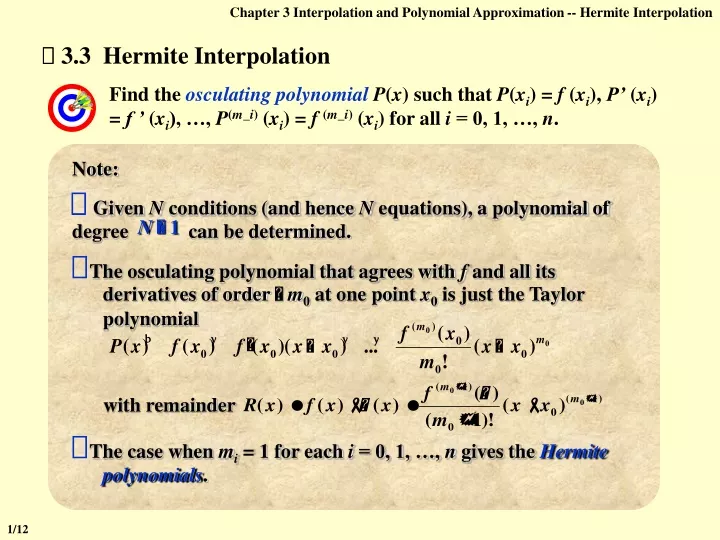
Chapter 3 Interpolation and Polynomial Approximation -- Hermite Interpolation. Find the osculating polynomial P ( x ) such that P ( x i ) = f ( x i ), P’ ( x i ) = f ’ ( x i ), …, P ( m_i ) ( x i ) = f ( m_i ) ( x i ) for all i = 0, 1, …, n.

E N D
Chapter 3 Interpolation and Polynomial Approximation -- Hermite Interpolation Find the osculating polynomialP(x) such that P(xi) = f (xi), P’ (xi) = f ’ (xi), …, P(m_i) (xi) = f(m_i) (xi) for all i = 0, 1, …, n. The osculating polynomial that agrees with f and all its derivatives of order m0 at one point x0 is just the Taylor polynomial with remainder 3.3 Hermite Interpolation Note: Given N conditions (and hence N equations), a polynomial of degree can be determined. N 1 The case when mi= 1 for each i = 0, 1, …, n gives the Hermite polynomials. 1/12
Chapter 3 Interpolation and Polynomial Approximation -- Hermite Interpolation Similar to Lagrange error analysis = 0 i where hi(xj) = ij , hi’(x1) = 0, (xi) = 0, ’(x1) = 1 2 = + P ( x ) f ( x ) h ( x ) f ’ ( x1 ) h ( x ) 3 1 i i = - - 2 h ( x ) C ( x x ) ( x x ) 0 0 1 2 h1 h1 h1 h1 h1 = + - - h ( x ) ( Ax B )( x x )( x x ) 1 0 2 (x) = - - - ( x ) C ( x x )( x x )( x x ) 1 0 1 2 ’(x1) = 1 C1can be solved. Example: Supposex0 x1 x2. Given f(x0), f(x1), f(x2) and f ’(x1), find the polynomial P(x) such that P(xi) = f (xi),i = 0, 1, 2, and P’(x1) = f ’(x1). Analyze the errors. Solution: First of all, the degree of P(x) must be … 3. Similar to Lagrange polynomials, we may assume the form of Hermite polynomial as x1, x2, andh0’(x1) = 0 x1is a multiple root. Has roots h0(x) h0(x0) = 1 C0 h2(x) Similar to h0(x). Has roots x0, x2 h1(x) A and Bcan be solved with h1(x1) = 1 and h1’(x1) = 0. Has roots x0, x1, x2 2/12
Chapter 3 Interpolation and Polynomial Approximation -- Hermite Interpolation n n + = H2n+1 yi h ( x ) yi’ h ( x ) ( x ) i i = = 0 0 i i where hi(xj) = ij, hi’(xj) = 0, (xj) = 0, ’(xj) = ij x0, …, xi , …, xn are all roots with multiplicity 2 = + h ( x ) ( A x B ) ( x ) L2 i i i n, i hi hi hi hi hi hi = - ( x ) C ( x x ) Ln, i2(x) i i (x) ’(xi) = 1 Ci= 1 = ( x ) - ( x x ) Ln, i2(x) i If , then In general, given x0, …, xn; y0, …, ynand y0’, …, yn’. The Hermite polynomial H2n+1(x) satisfies H2n+1(xi) = yi and H’2n+1(xi) = yi’ for all i. Solution: Let hi(x) Aiand Bi can be solved by hi(xi) = 1 and hi’(xi) = 0 Such a Hermite interpolating polynomial is unique All the roots x0, …, xnhave multiplicity 2 except xi 3/12
Chapter 3 Interpolation and Polynomial Approximation -- Hermite Interpolation Quiz:Givenxi = i +1, i = 0, 1, 2, 3, 4, 5.Which one is h2(x)? y y 1 - 1 - - 0.5 0.5 - x 0 1 2 3 4 5 6 - x 0 1 2 3 4 5 6 slope=1 HW: p.140 #7 4/12
Chapter 3 Interpolation and Polynomial Approximation -- Cubic Spline Interpolation Example: Consider the Lagrange polynomial Pn(x) of on [5, 5]. Take Pn(x) f (x) 2.5 2 1.5 1 0.5 Piecewise polynomial approximation 0 - 0.5 - 5 - 4 - 3 - 2 - 1 0 1 2 3 4 5 3.4 Cubic Spline Interpolation Remember what I have said? Increasing the degree of interpolating polynomial will NOT guarantee a good result, since high-degree polynomials are oscillating. 5/12
Chapter 3 Interpolation and Polynomial Approximation -- Cubic Spline Interpolation Approximate f (x) by linear polynomials on each subinterval : uniform Let . Then as No longer smooth. Given Construct the Hermite polynomial of degree 3 with y and y’ on the two endpoints of . It is not easy to obtain the derivatives. Piecewise linear interpolation How can we make a smooth interpolation without asking too much from f ? Headache … Hermite piecewise polynomials 6/12
Chapter 3 Interpolation and Polynomial Approximation -- Cubic Spline Interpolation Cubic Spline Definition: Given a function f defined on [a, b] and a set of nodes a = x0 < x1 < … < xn = b, a cubic spline interpolantS for f is a function that satisfies the following conditions: • S(x) is a cubic polynomial, denoted Si(x), on the subinterval • [ xi , xi+1] for each i = 0, 1, …, n – 1; • S(xi) = f (xi) for each i = 0, 1, …, n; • Si+1(xi+1) = Si(xi+1) for each i = 0, 1, …, n – 2; • S’i+1(xi+1) = S’i(xi+1) for each i = 0, 1, …, n – 2; • S”i+1(xi+1) = S”i(xi+1) for each i = 0, 1, …, n – 2; H(x) f(x) S(x) 7/12
Chapter 3 Interpolation and Polynomial Approximation -- Cubic Spline Interpolation - - x x x x - 1 j j + M M - 1 j j h h j j - - 2 2 ( x x ) ( x x ) Sj’(x) = - 1 j j - + + M M A - - 1 1 j j j 2 h 2 h Can be solved by Sj(xj1) = yj1 Sj(xj) = yj j j - - 3 3 ( x x ) ( x x ) Sj(x) = - 1 j j + + + M M A x B - 1 j j j j 6 h 6 h j j Method of Bending Moment Let hj = xj– xj – 1 and S(x) = Sj(x) for x [ xj – 1, xj ]. The bending moment Then Sj”(x) is a polynomial of degree , which can be determined by the values of f on nodes. 1 2 Assume Sj”(xj1) = Mj1, Sj”(xj) = Mj. Then for all x [ xj – 1, xj ], For each j it is a cubic polynomial Sj”(x) = Integrate Sj”(x) twice, we obtain Sj’(x) and Sj(x) : 8/12
Chapter 3 Interpolation and Polynomial Approximation -- Cubic Spline Interpolation - - y y M M - - 1 1 j j j j = - A h j j h 6 j 6 = - m = - l - - - g ( f [ x , x ] f [ x , x ]) 2 2 ( x x ) ( x x ) M M 1 - - + - M x x M x 1 x 1 j j j j j - - + 1 1 j j j j - + + - j j h h M M f [ x , x ] h - - 1 1 j j j j + = - + - 2 2 + A x B ( y h ) ( y h ) - - 1 j j 1 1 j j j j j 2 h 2 h 6 - 1 j j j j j j 6 h 6 h j j j j - - - 2 2 ( x x ) ( x x ) M M - + + 1 1 j j j j + + - M M f [ x , x ] h j + + + 1 1 1 j j j j 2 h 2 h 6 + + 1 1 j j From Sj’(xj) = Sj+1’(xj), we can combine the coefficients for Mj1,Mj, and Mj+1. Define , , and h + 1 j l = m + + l = M 2 M M g j - + + 1 1 j j j j j j h h + 1 j j Now solve for Mj: Since S’is continuous at xj [xj1, xj]:Sj’(x) = [xj, xj+1]:Sj+1’(x) = for j 1 n1 That is, we have unknowns but only equations. n+1 n1 Extra 2 boundary conditions are needed. 9/12
Chapter 3 Interpolation and Polynomial Approximation -- Cubic Spline Interpolation - - 2 - 2 M M ( x x ) ( x a ) [ a, x1]:S1’(x) = - + + - 1 0 1 M M f [ x , x ] h 0 1 0 1 1 2 h 2 h 6 1 1 6 + = - = 2 M M ( f [ x , x ] ) g y0’ 0 1 0 1 0 h 1 6 - = + = f [ x , x ]) g M 2 M ( yn’ - - 1 n n n 1 n n h n Then S’(a) = y0’, S’(b) = yn’ /* Clamped boundary */ Similar for Sn’(x) on [ xn1, b] S”(a) = y0”=M0, S”(b) = yn”=Mn The case when M0 =Mn = 0 is called a free boundary, and when that occurs, the spline is called a Natural Spline. Periodic boundary: If f is a periodic function, that is, yn=y0and S’(a+) = S’(b) M0 =Mn 10/12
Chapter 3 Interpolation and Polynomial Approximation -- Cubic Spline Interpolation If f C[ a, b ] and . Then as max hi 0. Note: Cubic Spline can be uniquely determined by its boundary conditions as long as the coefficient matrix is strictly diagonally dominant. HW: p.153-154 #9, 17 That is, the accuracy of approximation can be improved by adding more nodes without increasing the degree of the splines. Sketch of the Algorithm: Cubic Spline ①Compute j , j , gj ; ②Solve for Mj ; ③Find the subinterval which contains x (i.e. find the corresponding j ); ④ Approximate f(x) by Sj(x). 11/12
Chapter 3 Interpolation and Polynomial Approximation -- Cubic Spline Interpolation Lab 06. Cubic Spline Time Limit: 1 second; Points: 4 Construct the cubic spline interpolant S for the function f, defined at points x0 < x1 < … < xn, satisfying some given boundary conditions. Partition an given interval into m equal-length subintervals, and approximate the function values at the endpoints of these subintervals. 12/12