Download
1 / 26
260 likes | 402 Views
Data Warehousing & OLAP. Chapter 25, Ramakrishnan & Gehrke (Sections 25.1-25.10). Introduction. Increasingly, organizations are analyzing current and historical data to identify useful patterns and support business strategies.

E N D
Data Warehousing & OLAP Chapter 25, Ramakrishnan & Gehrke (Sections 25.1-25.10)
Introduction • Increasingly,organizations are analyzing current and historical data to identify useful patterns and support business strategies. • Emphasis is on complex, interactive, exploratory analysis of very large datasets created by integrating data from across all parts of an enterprise; data is fairly static. • Contrast such On-Line Analytic Processing (OLAP) with traditional On-line Transaction Processing (OLTP): mostly long queries, instead of short update Xacts.
Three Complementary Trends • Data Warehousing: Consolidate data from many sources in one large repository. • Loading, periodic synchronization of replicas. • integration of operational OLTP databases. • integrate through conflicts in schemas, semantics, platforms, integrity constraints, etc. • data cleaning. • OLAP: • Complex SQL queries and views. • Queries based on spreadsheet-style operations and “multidimensional” view of data. • Interactive and “online” queries. • Data Mining: Exploratory search for interesting trends and anomalies. (not covered in this course.)
OLAP EXTERNAL DATA SOURCES Data Warehousing EXTRACT TRANSFORM LOAD REFRESH • Integrated data spanning long time periods, often augmented with summary information. • Several gigabytes to terabytes common. • Interactive response times expected for complex queries; ad-hoc updates uncommon. updates typically batched. currency compromised. DATA WAREHOUSE Metadata Repository SUPPORTS DATA MINING
Warehousing Issues • Semantic Integration: When getting data from multiple sources, must eliminate mismatches, e.g., different currencies, schemas. • Heterogeneous Sources: Must access data from a variety of source formats and repositories. • Replication capabilities can be exploited here. • Load, Refresh, Purge: Must load data, periodically refresh it, and purge too-old data. Whether we purge or not depends on application. • Metadata Management: Must keep track of source, loading time, and other information for all data in the warehouse. – Data Provenance.
8 10 10 pid 11 12 13 30 20 50 25 8 15 1 2 3 timeid Multidimensional Data Model timeid sales locid pid • Collection of numeric measures, which depend on a set of dimensions. • E.g., measure Sales, dimensions Product (key: pid), Location (locid), and Time (timeid). Slice locid=1 is shown: locid
MOLAP vs ROLAP • Multidimensional data can be stored physically in a (disk-resident, persistent) array; called MOLAP systems. Alternatively, can store as a relation; called ROLAP systems. In MOLAP, combo. of dimension values directly mapped to addresses. • compression and sparsity issues. • The main relation, which relates dimensions to a measure, is called the fact table. Each dimension can have additional attributes and an associated dimension table. • E.g., Products(pid, pname, category, price) • Fact tables are much larger than dimensional tables.
Dimension Hierarchies • For each dimension, the set of values can be organized in a hierarchy: PRODUCT TIME LOCATION year quarter country category week month state pname date city Hierarchy schema
Modeling of Dimensions • Star schema: table per dimension. • simplicity: each dimension (hierarchy modeled in one table). • easier to formulate queries (one join/dimension). • poor modeling capabilities: what if dimension hierarchy is unbalanced and/or heterogeneous? • Snowflake schema: table per level of hierarchy per dimension. • more flexibility than star schema. • but heterogeneous dimension hierarchies still problematic. • Query formulation inherently more complex. (How many joins/dimension?).
OLAP Queries • Influenced by SQL and by spreadsheets. • A common operation is to aggregate a measure over one or more dimensions. • Find total sales. • Find total sales for each city, or for each state. • Find top five products ranked by total sales. • Find top 10 products that accounted for max. proportion of sales in the Northeast, ranked in order of proportion. • Find the top performing region for a gn. product, and find the city in the region which accounts for less than 10% toward the region’s total performance on the product. • Roll-up: Aggregating at different levels of a dimension hierarchy. • E.g., Given total sales by city, we can roll-up to get sales by state.
OLAP Queries • Drill-down: The inverse of roll-up. • E.g., Given total sales by state, can drill-down to get total sales by city. • E.g., Can also drill-down on different dimension to get total sales by product for each state. • Pivoting: Aggregation on selected sets of dimensions plus rendering. • E.g., Pivoting on Location and Time yields this cross-tabulation: BC QC Total 63 81 144 1995 • Slicing and Dicing:Equality • and range selections on one • or more dimensions. 38 107 145 1996 75 35 110 1997 176 223 339 Total
Comparison with SQL Queries SELECT T.year, L.state, SUM(S.sales) FROM Sales S, Times T, Locations L WHERE S.timeid=T.timeid AND S.timeid=L.timeid GROUP BYT.year, L.state • The cross-tabulation obtained by pivoting can also be computed using a collection of SQLqueries: SELECT T.year, SUM(S.sales) FROM Sales S, Times T WHERE S.timeid=T.timeid GROUP BYT.year SELECT L.state, SUM(S.sales) FROM Sales S, Location L WHERE S.timeid=L.timeid GROUP BY L.state Plus of course, the GROUP BY nothing query on Sales.
The CUBE Operator • Generalizing the previous example, if there are k dimensions, we have 2^k possible SQL GROUP BY queries that can be generated through pivoting on a subset of dimensions. (This ignores possibilities afforded by dimension hierarchies.) • E.g.: CUBE BY pid, locid, timeid SUM(Sales) • Equivalent to rolling up Sales on all eight subsets of the set {pid, locid, timeid}; each roll-up corresponds to a SQL query of the form: SELECT …, SUM(S.sales) FROM Sales S GROUP BY grouping-list Lots of recent work on optimizing the CUBE operator!
CUBE • Why a new operator (for cube)? • CUBE’s value is in affording efficient computation for multiple granularity aggregates by sharing work (e.g., passes over fact table, previously computed aggregates, etc.). • CUBE is expensive to compute and is huge. • CUBE may be partly or fullymaterialized, or not at all. • Tremendous interest in: • computing it fast. • compressing it. • approximating it.
TIMES timeid date week month quarter year holiday_flag (Fact table) pid timeid locid sales SALES PRODUCTS LOCATIONS pid pname category price locid city state country Design Issues • Fact table in BCNF; dimension tables not normalized. • Dimension tables are small; updates/inserts/deletes are relatively less frequent. So, anomalies less important than good query performance. • This kind of schema is very common in OLAP applications, and is called a star schema; computing the join of all these relations is called a star join. (Recall the alternative organization – snowflake schema.) • Neither schema fully satisfactory for OLAP apps.
Implementation Issues • New indexing techniques: Bitmap indexes, Join indexes, array representations, compression, precomputation of aggregations, etc. • E.g., Bitmap index: sex custid name sex rating rating Bit-vector: 1 bit for each possible value. Many queries can be answered using bit-vector ops! F M Bitmap indexes elaborated elsewhere.
Join Indexes • Consider the join of Sales, Products, Times, and Locations, possibly with additional selection conditions (e.g., country=“Canada”). • A join index can be constructed to speed up such joins. The index contains [s,p,t,l] if there are tuples (with rid) s in Sales, p in Products, t in Times and l in Locations that satisfy the join (and selection) conditions. p, t, l could instead be values satisfying selections in those tables. • Problem: Number of join indexes can grow rapidly. • A variant of the idea addresses this problem: For each column with an additional selection (e.g., country), build an index with [c,s] in it if a dimension table tuple with valuec in the selection column joins with a Sales tuple with rids; if indexes are bitmaps, called bitmapped join index. E.g., bit vectors BM(Canada), BM(USA), etc. These might be organized by another index on Country, e.g., by a B+tree.
Bitmapped Join Index TIMES timeid date week month quarter year holiday_flag (Fact table) • Consider a query with conditions price=10 and country=“Canada”. Suppose tuple (with sid) s in Sales joins with a tuple p with price=10 and a tuple l with country =“Canada”. There are two join indexes (one each for [Product,Sales] and [Location,Sales]; one containing [10,s] and the other [Canada,s]. • Intersecting these indexes tells us which tuples in Sales are in the join and satisfy the given selection. pid timeid locid sales SALES PRODUCTS LOCATIONS pid pname category price locid city state country
Views and Decision Support • OLAP queries are typically aggregate queries. • Precomputation is essential for interactive response times. • The CUBE is in fact a collection of aggregate queries, and precomputation is especially important: lots of work on what is best to precompute given a limited amount of space to store precomputed results. • Warehouses can be thought of as a collection of asynchronously replicated tables and periodically maintained views. • Has renewed interest in view maintenance!
View Modification (Evaluate On Demand) CREATE VIEWRegionalSales(category,sales,state) ASSELECT P.category, S.sales, L.state FROM Products P, Sales S, Locations L WHERE P.pid=S.pid AND S.locid=L.locid View SELECT R.category, R.state, SUM(R.sales) FROMRegionalSales R GROUP BYR.category, R.state Query SELECT R.category, R.state, SUM(R.sales) FROM (SELECT P.category, S.sales, L.state FROM Products P, Sales S, Locations L WHERE P.pid=S.pid AND S.locid=L.locid) R GROUP BY R.category, R.state Modified Query
View Materialization(Precomputation) • Suppose we precompute RegionalSales and store it with a clustered B+ tree index on [category,state,sales]. • Then, previous query can be answered by an index-only scan (i.e., index scan). • The bottom queries (try to) use index probe. SELECT R.state, SUM(R.sales) FROM RegionalSales R WHERE R.category=“Printer” GROUP BY R.state SELECT R.category, SUM(R.sales) FROM RegionalSales R WHERE R. state=“BC” GROUP BY R.category Index on precomputed view is great! Index is less useful (must scan entire leaf level).
Issues in View Materialization • What views should we materialize, and what indexes should we build on the precomputed results? • Given a query and a set of materialized views, can we use the materialized views to answer the query? • How frequently should we refresh materialized views to make them consistent with the underlying tables? (And how can we do this incrementally?)
Interactive Queries: Beyond Materialization • Top N Queries: If you want to find the 10 (or so) cheapest cars, it would be nice if the DB could avoid computing the costs of all cars before sorting to determine the 10 cheapest. • Idea: Guess at a cost c such that the 10 cheapest all cost less than c, and that not too many more cost less. Then add the selection cost < c and evaluate the query. • If the guess is right, great, we avoid computation for cars that cost more than c. • If the guess is wrong, need to reset the selection and recompute the query.
Top N Queries SELECT P.pid, P.pname, S.sales FROM Sales S, Products P WHERE S.pid=P.pid AND S.locid=1 AND S.timeid=3 ORDER BY S.sales ASC OPTIMIZE FOR 10 ROWS • OPTIMIZE FOR construct is not in SQL:1999! • Cut-off value c is chosen by optimizer. SELECT P.pid, P.pname, S.sales FROM Sales S, Products P WHERE S.pid=P.pid AND S.locid=1 AND S.timeid=3 AND S.sales < c ORDER BY S.sales ASC
Interactive Queries: Beyond Materialization • Online Aggregation: Consider an aggregate query, e.g., finding the average sales by state. Can we provide the user with some information before the exact average is computed for all states? • Can show the current “running average” for each state as the computation proceeds. • Even better, if we use statistical techniques and sample tuples to aggregate instead of simply scanning the aggregated table, we can provide bounds such as “the average for BC is 2000±102 with 95% probability. • Should also use nonblocking algorithms! • Has exciting new applications – streaming data, sensor data, etc.
Summary • Decision support is an emerging, rapidly growing subarea of databases. • Involves the creation of large, consolidated data repositories called data warehouses. • Warehouses exploited using sophisticated analysis techniques: complex SQL queries and OLAP “multidimensional” queries (influenced by both SQL and spreadsheets). • New techniques for database design, indexing, view maintenance, and interactive querying need to be supported.