Download
1 / 40
440 likes | 629 Views
Course details Instructor: Oliver Fringer, Dept. of Civil and Environmental Engineering, Terman Bldg. Room M17, fringer@stanford.edu TA: Vivien Chua, vchua@stanford.edu Office hours: 1:00-4:00 pm F Course web page: fluid.stanford.edu/~fringer/teaching/cee262c

E N D
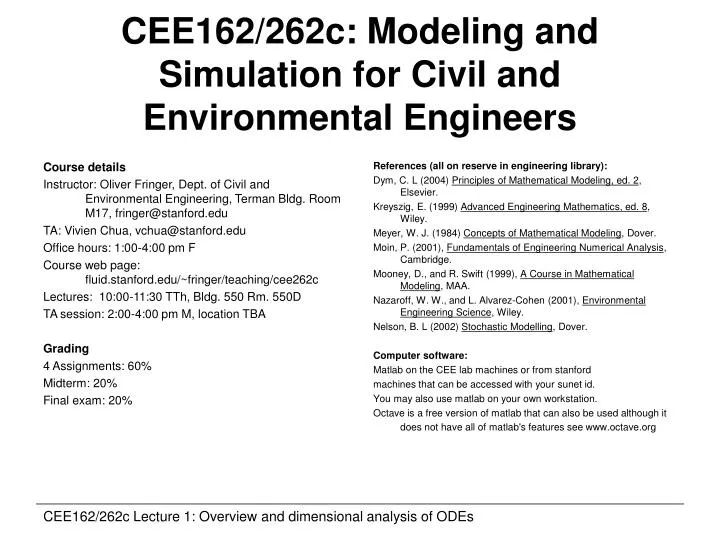
Course details Instructor: Oliver Fringer, Dept. of Civil and Environmental Engineering, Terman Bldg. Room M17, fringer@stanford.edu TA: Vivien Chua, vchua@stanford.edu Office hours: 1:00-4:00 pm F Course web page: fluid.stanford.edu/~fringer/teaching/cee262c Lectures: 10:00-11:30 TTh, Bldg. 550 Rm. 550D TA session: 2:00-4:00 pm M, location TBA Grading 4 Assignments: 60% Midterm: 20% Final exam: 20% CEE162/262c: Modeling and Simulation for Civil and Environmental Engineers References (all on reserve in engineering library): Dym, C. L (2004) Principles of Mathematical Modeling, ed. 2, Elsevier. Kreyszig, E. (1999) Advanced Engineering Mathematics, ed. 8, Wiley. Meyer, W. J. (1984) Concepts of Mathematical Modeling, Dover. Moin, P. (2001), Fundamentals of Engineering Numerical Analysis, Cambridge. Mooney, D., and R. Swift (1999), A Course in Mathematical Modeling, MAA. Nazaroff, W. W., and L. Alvarez-Cohen (2001), Environmental Engineering Science, Wiley. Nelson, B. L (2002) Stochastic Modelling, Dover. Computer software: Matlab on the CEE lab machines or from stanford machines that can be accessed with your sunet id. You may also use matlab on your own workstation. Octave is a free version of matlab that can also be used although it does not have all of matlab's features see www.octave.org CEE162/262c Lecture 1: Overview and dimensional analysis of ODEs
Real world/Problem of interest Question Model Data Theory Simulation General picture of modeling Compare/Verify Prediction/Explanation Result CEE162/262c Lecture 1: Overview and dimensional analysis of ODEs
Verification is key Complex models can be difficult to verify (e.g. "model has many bells and whistles but there is no guarantee that they all work") Simple models can be restrictive (e.g. "this model works for this case only") Problem vs. Model Complexity Simple model for a complex problem. Complex model for a complex problem. Harder Typical problem? Problem/abstraction Complexity Simple model for a simple problem. Complex model for an easy problem. Model Complexity/Resolution Harder CEE162/262c Lecture 1: Overview and dimensional analysis of ODEs
Basic Modeling Ideas • Dimensional analysis • Scaling • Will the model scale up/down? • Resolution • How detailed does the answer need to be? • Conservation principles • Resource constraints CEE162/262c Lecture 1: Overview and dimensional analysis of ODEs
Types of Models • Descriptive (predict a result) vs. Prescriptive (optimize for a given set of conditions) • Linear vs. nonlinear • Discrete vs. continuous • Deterministic vs. stochastic • Empirical vs. analytical CEE162/262c Lecture 1: Overview and dimensional analysis of ODEs
Dimensional Analysis and ODEs Overview • Dimensional analysis • Buckingham Pi theorem • Nondimensionalization of an ODE • Analytical solution of a linear ODE using an integrating factor • Numerical solution of a nonlinear ODE (only showing the results) • Linearization of the nonlinear ODE and obtaining an approximate linearized solution References: Dym, Ch 2; Mooney & Swift, Ch 5; Kreyszig, Ch 2 CEE162/262c Lecture 1: Overview and dimensional analysis of ODEs
Dimensional analysis • Dimensional analysis seeks to describe a phenomenon based on dimensional arguments alone [V] = L/T [r]=M/L3 [h] = L [m] = M [d] = L [g] = L/T2 Write V in terms of the other parameters: [V]2 = [g][h] r d m height h V (velocity) g CEE162/262c Lecture 1: Overview and dimensional analysis of ODEs
Buckingham Pi Theorem • Given a set of n dimensional parameters defined by m fundamental dimensions, we can define the behavior of the system in terms of a single relationship among n-m nondimensional variables • Dimensional parameters: • Nondimensional parameters: CEE162/262c Lecture 1: Overview and dimensional analysis of ODEs
Dimensional analysis of the bouncing ball problem • Eight parameters, n=8 • m=3 fundamental dimensions, m=3. • n-m=5 nondimensional parameters. CEE162/262c Lecture 1: Overview and dimensional analysis of ODEs
Computing the nondimensional parameters: • Choose m dimensional variables that contain all of the dimensions involved, i.e. Mass, Length, Time (M,L,T): • Write down the nondimensional numbers as a product of these m dimensional variables and the remaining n-m dimensional variables: • Solve for the powers that make the parameters dimensionless. CEE162/262c Lecture 1: Overview and dimensional analysis of ODEs
We can almost always determine the powers without any algebra • From this we know that CEE162/262c Lecture 1: Overview and dimensional analysis of ODEs
Practical Buckingham Pi • Choose m dimensional variables that contain all of the dimensions involved, i.e. Mass, Length, Time (M,L,T): • Create M, L, T scales from these three variables: • Use these three to nondimensionalize the remaining 5: CEE162/262c Lecture 1: Overview and dimensional analysis of ODEs
Interpreting nondimensional variables • Nondimensional lengths: • Nondimensional on its own: CEE162/262c Lecture 1: Overview and dimensional analysis of ODEs
Interpreting nondimensional variables • In terms of forces: • In terms of time scales: CEE162/262c Lecture 1: Overview and dimensional analysis of ODEs
Interpreting nondimensional variables • In terms of forces: • In terms of mass scales: CEE162/262c Lecture 1: Overview and dimensional analysis of ODEs
Deriving relationships empirically • Fix these: • Perform experiments to relate these: Plot same data a different way: d is no longer relevant! CEE162/262c Lecture 1: Overview and dimensional analysis of ODEs
Can theory explain empirical result? CEE162/262c Lecture 1: Overview and dimensional analysis of ODEs
Modeling the effects of drag • The balance of forces on a falling ball is given by V CEE162/262c Lecture 1: Overview and dimensional analysis of ODEs
Nondimensionalize CEE162/262c Lecture 1: Overview and dimensional analysis of ODEs
CEE162/262c Lecture 1: Overview and dimensional analysis of ODEs
CEE162/262c Lecture 1: Overview and dimensional analysis of ODEs
CEE162/262c Lecture 1: Overview and dimensional analysis of ODEs
Tennis Ball dropped from 1 m in air P4 = 3192 Buoyant force is 3200 times larger than viscous force on ball. P5 = 170 Ball weighs 170 times more than the buoyant force. CEE162/262c Lecture 1: Overview and dimensional analysis of ODEs
CEE162/262c Lecture 1: Overview and dimensional analysis of ODEs
Comparing the two models (after dropping the primes and assuming dy/dt<0, a3<< a2) Viscosity/Weight Linear, constant coefficients inhomogeneous Nonlinear, constant coefficients inhomogeneous Pressure/Weight We can solve the linear equation analytically. CEE162/262c Lecture 1: Overview and dimensional analysis of ODEs
Solution of the linear ODE CEE162/262c Lecture 1: Overview and dimensional analysis of ODEs
CEE162/262c Lecture 1: Overview and dimensional analysis of ODEs
Solution for the falling ball: CEE162/262c Lecture 1: Overview and dimensional analysis of ODEs
Result of plotting The solution with small a1 cannot be plotted because the effect of roundoff error is too large when written in this way. CEE162/262c Lecture 1: Overview and dimensional analysis of ODEs
We can use the Taylor series to determine the limiting case of a1=0: CEE162/262c Lecture 1: Overview and dimensional analysis of ODEs
CEE162/262c Lecture 1: Overview and dimensional analysis of ODEs
System of equations and its numerical solution bounce.m CEE162/262c Lecture 1: Overview and dimensional analysis of ODEs
bouncealpha.m Decreasing CEE162/262c Lecture 1: Overview and dimensional analysis of ODEs
bouncealpha.m CEE162/262c Lecture 1: Overview and dimensional analysis of ODEs
Linearization about a known solution CEE162/262c Lecture 1: Overview and dimensional analysis of ODEs
CEE162/262c Lecture 1: Overview and dimensional analysis of ODEs
CEE162/262c Lecture 1: Overview and dimensional analysis of ODEs
CEE162/262c Lecture 1: Overview and dimensional analysis of ODEs
Overview of the regular perturbation expansion CEE162/262c Lecture 1: Overview and dimensional analysis of ODEs
CEE162/262c Lecture 1: Overview and dimensional analysis of ODEs