Download
1 / 20
220 likes | 354 Views
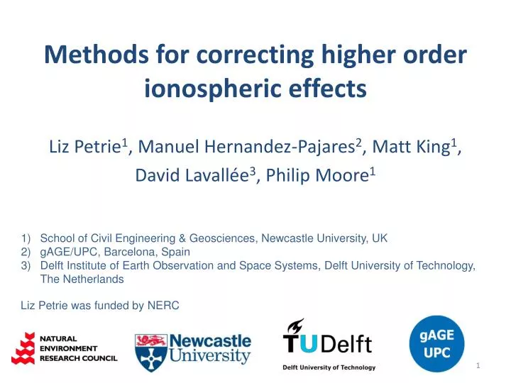
Methods for correcting higher order ionospheric effects. School of Civil Engineering & Geosciences, Newcastle University, UK gAGE /UPC, Barcelona, Spain Delft Institute of Earth Observation and Space Systems, Delft University of Technology, The Netherlands.

E N D
Methods for correcting higher order ionospheric effects School of Civil Engineering & Geosciences, Newcastle University, UK gAGE/UPC, Barcelona, Spain Delft Institute of Earth Observation and Space Systems, Delft University of Technology, The Netherlands Liz Petrie1, Manuel Hernandez-Pajares2, Matt King1, David Lavallée3, Philip Moore1 Liz Petrie was funded by NERC
Why? • Higher order effects not removed when using ‘ionosphere-free’ linear combination • Long term cycles in ionospheric activity 60 Change in the Earth’s mean Total Electron Content (TEC) since 1995 50 40 Centre for Orbit Determination in Europe (CODE) Mean TEC /TECU 30 http://aiuws.unibe.ch/ionosphere/meantec.gif 20 10 2007 1996 Time / Years
Expansion of ionospheric refractive index dTEC bending term Geometric bending term I2 I3 I4+ order - negligible Higher order ionospheric terms
θ θ Ionospheric effects • 1st order phase delay • 2nd order phase delay • 3rd order phase delay cosθ +ve GPS signal magnetic field cosθ - ve
Processing • GPS reprocessing: 5 comparison runs I2 and I3 modelled I2 only modelled I2,I3 and bending modelled Without higher order effects ‘Base’ ‘IGRF’ ‘IGRF2’ ‘Bending’ Hoque & Jakowski (2008) empirical formulae used ‘Dipole’ • Strategy • 60 sites in a global fiducial-free network • GAMIT v10.35 (adapted) • odd days during 1995-2008 • VMF1 troposphere mapping functions • absolute antenna phase center offsets • met files/VMF1 for a priori zenith hydrostatic delay • sub-daily atmospheric loading
Effect of I2 and I3 TECU mm ‘Base’-‘IGRF’ 7 day Gaussian smoothing Data in Petrie et al. (2010) J Geophys Res 115(B3): B03417 90 day Gaussian smoothing
Effect of I2 and I3 Mean coordinate differences 2000.0-2003.0 Sites shown have at least 2.5 years of data. ‘IGRF’-‘Base’ Petrie et al. (2010) J. Geophys. Res. 115(B3): B03417
Effect of I2 and I3 ‘Base’-‘IGRF’ 1996.0-2001.0 2001.0-2006.0 0.0 to 0.29 mm yr -1 -0.34 to 0.0 mm yr -1. Petrie et al. (2010) J. Geophys. Res. 115(B3): B03417
I2 – effect of magnetic field model Magnetic field strength % difference (IGRF-dipole)/IGRF decimal date 2003.83 ‘Dipole’-‘IGRF’ 2001 - 2003 Petrie et al. (2010) J. Geophys. Res. 115(B3): B03417
Effect of I3 Reference frame mm ppb ‘Base’-‘IGRF’ ‘Base’-‘IGRF2’ ‘IGRF2’-‘IGRF’ Petrie et al. (2010) J. Geophys. Res. 115(B3): B03417
Effect of bending terms mm ppb ‘Base’-‘IGRF’ ‘Base’-‘Bending’ ‘Bending’-‘IGRF’ Petrie, E. J. et al. (2010) J. Geod. (online).
Effect of bending terms GOLD IISC Mean coordinate differences 2001.0-2004.0 Sites shown have at least 2.5 years of data. MAW1 (of 2001) Petrie, E. J. et al. (2010) J. Geod. (online).
value at shell height / average value / integrated along signal I2 shell height (location of pierce point) Evaluate as B.k or Bcosθ mapping function dipole/IGRF /other model magnetic field from models / maps of VTEC e.g. IONEX files solved from GPS STEC Factors affecting I2 e.g. 450km
Pierce point hi = e.g. 450 km Layer / ‘thin shell’ ‘Earth surface’ (spherical) O Some remaining issues • source of STEC • height of magnetic field evaluation
STEC from maps Height of peak electron density at 270° longitude, DOY 301, 2001, based on IRI2007 Variations in estimated VTEC with varying thin layer height, hi, based on: - STECof 350TECU - 10 degrees elevation Petrie et al. (2010) J. Geod. (online).
Effect of STEC source? ‘Dipole’-‘Base’ 2001.0-2004.0 2001.0-2004.0 Steigenberger et al. (2006) J. Geophys. Res. Petrie et al. (2010) J. Geophys. Res. DOY 100, 2002 to DOY 365, 2003 Hernández-Pajares et al. (2007) J. Geophys. Res.
Magnetic field – changing shell height DARW (12.84S, 131.13E), DOY 301, 2001. 250km 300km 350km 400km 450km 500km Height values plotted Difference of I2 to value at 450 km
Summary • Neglecting higher order ionospheric effects bias of up to ~ 0.34 mm/yr rates, ~ 10mm Z-translation • Effect of IGRF/dipole < 1mm (mean coordinates) • I3 term only limited effect • Bending terms • trial implementation: seem to be absorbed by TZDs • Solar activity is currently increasing towards the next ionospheric maximum
Expansion of ionospheric refractive index ∫ Ne2 (shape factor, Nm) I4+ order - negligible I1 dTEC bending term I2 I3 Geometric bending term fixed height/ variable value at shell height / average value / integrated along signal shell height (location of pierce point) hmF2 interpolate / ionospheric model Nm Evaluate as B.k or Bcosθ mapping function from models / maps of VTEC e.g. IONEX files solved from GPS dipole/IGRF /other model magnetic field STEC