Download

1 / 78
930 likes | 1.23k Views
Uncertainty on Hydrological Models in Climate Change Scenarios. S. Jamshid Mousavi Associate Professor, Civil Engineering Department, Amirkabir University of Technology (Polytechnic of Tehran), Tehran, Iran jmosavi@aut.ac.ir Regional Asian G-WADI Workshop, June 2011, Tehran, Iran.

E N D
Uncertainty on Hydrological Models in Climate Change Scenarios S. JamshidMousavi Associate Professor, Civil Engineering Department, Amirkabir University of Technology (Polytechnic of Tehran), Tehran, Iran jmosavi@aut.ac.ir Regional Asian G-WADI Workshop, June 2011, Tehran, Iran
Steps in climate change impact studies • Uncertainty in climate change studies • Hydrological models and uncertainty sources • Uncertainty-based calibration/simulation of • hydrological models • Successive uncertainty fitting (SUFI) approach • Uncertainty-based calibration of HEC-HMS • model: Tamar Basin experience • Uncertainty-based calibration of SWAT model: Karkheh River Basin experience • Climate-change-driven runoff simulation and water allocation at basin scale: Karkheh River Basin experience Outline
Typical steps of climate change impact studies on water resources Emission scenarios 1-Select a few number of emission scenarios 2-Take GCMs outputs of metrological variables 3-Downscale the output of the GCMs 4-Build a calibrated hydrological model of the basin 5-Simulate hydrologic variables of interest (runoff) subject to downscaled climate-change-driven inputs 6-Extend the study chain to water management system GCM outputs Precipitation, temperature, etc Downscaling Downscaled precipitation, temperature, etc Calibrated hydrological model CC-driven simulated runoff scenarios Management and water allocation model
Uncertainty Issue • Uncertainty on future emission of green gasses: Emission scenarios • Uncertainty on nature of ocean-atmosphere physical processes and so structure of GCMs • Uncertainty related to quantification of regional and local effects reflected in downscaling models • Uncertainty on hydrological models • Uncertainty on behavior of complex socio-economic and management systems
Approaches to deal with uncertainty • Scenario generation-based techniques • Techniques based on probabilistic representation of processes involved (e.g. Reliability Ensemble Averaging [Giorgi and Mearns 2002], Bayesian-based Multi-model Ensembles of GCMs [Tebaldi et al. 2005], …)
Uncertainty on Hydrological Models • Sources of uncertainty: • 1- Structural uncertainty • 2- Data uncertainty • 3- Parameter uncertainty Input Output processing Runoff Precipitation Hydrologic Modeling Watershed Unknown known
Calibration • Model parameters are determined through model calibration, because parameters may not have exact physical meaning or may not be easily measurable • Manual Calibration: • Trial and error-based parameter estimation procedure • Time consuming • Depends on expertise and judgment of the modeler • Does not account for uncertainty Automatic Calibration: • Systematic search procedures for finding parameter values • The search procedure is guided based on an objective function measuring how well any set of parameters perform 7 16
Calibration procedure Rainfall-precipitation data Parameter Estimation start Simulation in HEC-HMS Better Estimation of parameters Compare Hydrograph End Yes Error? NO 17
Difficulties with (Automatic) Calibration Techniques • Model uncertainty because of imperfect model structure due to either parameters interdependence or conceptual simplifications of physical processes taken place in real natural systems • Input uncertainty due to erroneous or approximate input data (Extending point rain data to areal data) • Parameter uncertainty andnonuniqunessdue tonon-identifiabilityfeature a) different parameter sets may not give rise to different model outputs resulting in parameternonuniquness ininverse-type problems b) model response surface can be insensitive to a number of parameters in the region of optimum solution • Multiple convergence regions and local optima solutions • Nonconvex shape of the response surface with discontinuous long curved ridges 9
Quality of Calibration Results Depend on: • The conceptual base and structure of the CRR model • The modeling technique addressing different types of uncertainty depending on quality and quantity of information and data available • The power and robustness of the optimization algorithm • Performance criteria or objective function 10
Uncertainty-based Calibration of Hydrological Models • Automatic calibration techniques: • 1- Monte-Carlo • 2- Generalized likelihood uncertainty estimator (GLUE) • 3- Bayesian techniques • 4- Parasol • 5- Successive uncertainty fitting (SUFI)
SUFI Technique • Extensively used in calibration of SWAT hydrological model at continent, regional and basin scales
HMS-SUFI: Uncertainty-based Calibration Technique • Step 1. Select an objective function (RMSE in the current application) • More importance is given to some • desired discharges like the peak flow • Step 2. Define physically meaningful absolute minimum and maximum ranges for each parameter • Step 3. Carry out a sensitivity analysis with respect to parameters • Step 4. Assign an initial uncertainty range to each parameter used in the first round of Latin hypercube. These ranges are smaller than the absolute ranges • Step 5. Generate n different sets of parameter values using Latin Hypercube sampling technique • Step 6. Evaluate the objective function, g, for each of n generated sets(Run HEC-HMS n times) • Step 7: Calculate thesensitivity analysis matrix J, Hessian Matrix H, Covariance matrix C, and parametercorrelations matrix r • Step 8: Calculate uncertainty indicatorsP-factor, R-factor,.., and new parameter rangesbased on best parameter set and matrices C and … 13
Conceptual basis of SUFI Uncertainty Analysis Input parameters: (Uniform distribution) Output variables: (95% PPU) 14
Uncertainty Analysis using SUFI • R-factor : Measures model predictive uncertainty • P-factor: • Percent of observed data (runoff) locating within 95PPU bounds of simulated ones • br2 • r2:Correlation coefficient between measured and simulated values • b: Slope of regression line Uncertainty measures 95PPU: Uncertainty Bound as 95% of probability distribution R-factor : Measures total predictive uncertainty in terms of normalized sum of 95% PPU bounds
HMS-SUFI MODELCase Study:TamarSubbasin • One of the basins ofGorganrood River located in the North west of Khorasan province in Iran. • Area of Gorganrood River52826 square kilometers • Area of Tamar basin about 1530 square kilometers • Considered important because of experiencing severe floods . 16 16
Gorgan-Roud Basin 17 17
Case Study-Tamar Subbasin • Lack of sufficient data at hydrometric and rainfall stations makes modeling the basin’s response to floods challenging • 4reliable flood events were available the first 3 of which were used for calibration and the last one for verification 18 18
Observed Flood Events Date, peak flow and duration of flood events 19 19
Hydrograph of first event Time 0 equals to (19Sep2004, 18:00) 20 20
Hydrograph of Second event Time 0 equals to (06May2005, 01:00) 21 21
Hydrograph of Second event Time 0 equals to (09Aug2005, 20:00) 22 22
Hydrograph of Second event Time 0 equals to (08Oct2005, 23 23
HEC-HMS Structure HEC-HMS Components Basin module Control Specification Meteorological module Transformation module Loss module Routingmodule Base flow module 8 24
BASIN MODULE Basin Module 25 25
Model of Tamar Basin in HEC-HMS • Divided into 7sub-basin with3routing reaches • SCS-CN Method Estimating hydrologic losses • Clark Method Transforming rainfall to runoff • Flood routing in reaches Muskingum method. • No base flow 26 26
Tamar Basin in HEC-HMS 27 27
Calibration Parameters • Loss method: SCS-CN Method 1- Curve number: 7 parameters (1 for each subbasin) 2- Initial abstraction: 7 parameters(1 for each subbasin) • Transformation Method: Clark 1-Time of concentration: estimated by SCS synthetic unit hydrograph approach 2- Storage Coefficient (R): • Routing Method: Muskingum (K,X) Total No. of Calibration Parameters=24 28 28
Manually-calibrated parameter values for each event and their upper and lower limits (suggested by IWRI (2008) 29
Results and AnalysisSingle-event Calibration Scenario-Event 1 30
Results and AnalysisSingle-event Calibration Scenarios-Events 2 and 3
Results and AnalysisJointly-calibrated events scenario with bigger weights assigned to Event 1 in the Obj. Function (Scenario 0W) 33
Results and AnalysisJointly-calibrated events with 31 parameters and increased Ia values of event-1 to 0.45 (Scenario 1) 34
Results and AnalysisJointly-calibrated events with 31 Parameters and decreased Ia values of event-3 to zero (Scenario 2) 35
Jointly-calibrated events with 31 Parameters and adjusted Ia values of event-1 and event-3 (Scenario 3) we were keen to see if there is another set of parameters with Ia values closer to initially-set bounds. The 31-parameter problem was run with Ialower bounds of event-1 as 0.35 (instead of 0.45 in scenario 6) and those of other events (1 and 2) as 0.05 (instead of zero in scenario 7). 36
Results and AnalysisNonuniqueness of Parameter Sets • The only difference between scenarios 1-3 is in their Ia lower and upper bounds • What about the other parameter values? Were they same? • Answer: No • Nonuniqueness 37
Verification Analysis Simulating Event 4 by 9 sets of Parameter Values Obtained in Calibration Stage Before recalibration of Ia After recalibration of Ia 38
Table 3. Simulated objective function and initial abstraction values of all recalibrated parameters Simulated objective function and Ia values of all recalibrated parameters (Screening Step)
Comparison of parameter values, other than Ia s, of the 6 screened parameter sets (See nonuniquness)
Dealing with UncertaintyUncertainty measures and the best obj. function obtained from another SUFI run with the new parameter bounds derived from 6 screened parameter sets : event 4 (values within parenthesis are for a smoothed hydrograph)
Parameter Bounds and Simulated Discharges in iterations 1 and 3 of SUFI with Newly-Selected Parameter Bounds:Event-4 42
Iteration’s 4 simulated discharges of the events in SUFI for jointly –calibrated eventswith fixed parameter intervals except initial abstraction ranges to find de-calibrated Ia values 45
ConclusionsThe proposed 3-stage procedure • 1- Obtain different parameter values by calibrating events either separately or jointly to come up with candidate parameter sets entering in verification stage • 2- Recalibrate the parameters reflecting initial basin conditions and then screen out the above candidate parameter sets based on how well they perform in verification and also how physically meaningful their recalibrated parameters are • 3- Calculate the new parameter ranges from the screened parameter values and re-run the SUFI model to find narrower parameter ranges, as the final parameter ranges, at which uncertainty indicators are still acceptable. Also check if the final ranges perform well in simulating all calibration events (Backward step). This needs again re-calibration of initial-basin-condition parameters with respect to calibration events 46
Karkheh River Basin Study 1- Climate Change Impact on Surface Runoff 2- Climate Impact on Water Allocation
Typical steps of climate change impact studies on water resources Emission scenarios 1-Select a few number of emission scenarios 2-Take GCMs outputs of metrological variables 3-Downscale the output of the GCMs 4-Build a calibrated hydrological model of the basin 5-Simulate hydrologic variables of interest (runoff) subject to downscaled climate-change-driven inputs 6-Extend the study chain to water management system GCM outputs Precipitation, temperature, etc Downscaling Downscaled precipitation, temperature, etc Calibrated hydrological model CC-driven simulated runoff scenarios Management and water allocation model
Karkheh River Basin ÷ Area: 4763592 Hectar • One of the most important basins in Iran in terms of Surface and groundwater resources, agriculture potential, hydropower generation,… • 16000 MCM of potential storage capacity 40% percent of which has been constructed
گGarsha Location of Dams in Karkheh Basin Tangmashoureh Koranbuzan Sazbon Seymareh ROR Karkeh Karkheh