Chapter 2 Parallel Programming background

1. Chapter 2 Parallel Programming background “By the end of this chapter, you should have obtained a basic understanding of how modern processors execute parallel programs & understand some rules of thumb for scaling performance of parallel applications.”

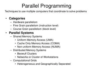
2. Traditional Parallel Models Serial Model • SISD Parallel Models • SIMD • MIMD • MISD* • S = Single • M = Multiple • D = Data • I = Instruction

3. Vocabulary & Notation (2.1) • Task vs. Data: tasks are instructions that operate on data; modify or create new • Parallel computation  multiple tasks • Coordinate, manage, • Dependencies • Data: task requires data from another task • Control: events/steps must be ordered (I/O)

4. Task Management – Fork-Join • Fork: split control flow, creating new control flow • Join: control flows are synchronized & merged

5. Graphical Notation – Fig. 2.1 Task Data Fork Join Dependency

6. Strategies (2.2) • Data Parallelism • Best strategy for Scalable Parallelism • P. that grows as data set/problem size grows • Split data set over set of processors with task processing each set • More Data  More Tasks

7. Strategies • Control Parallelism or • Functional Decomposition • Different program functions run in parallel • Not scalable – best speedup is constant factor • As data grows, parallelism doesn’t • May be less/no overhead

8. Regular vs. Irregular Parallelism • Regular: tasks are similar with predictable dependencies • Matrix multiplication • Irregular: tasks are different in ways that create unpredictable dependencies • Chess program • Many problems contain combinations

9. Hardware MechanisMS (2.3) Most important 2 • Thread Parallelism: implementation in HW using separate flow control for each worker – supports regular, irregular, functional decomposition • Vector Parallelism: implementation in HW with one flow control on multiple data elements – supports regular, some irregular parallelism

10. Branch statements Detrimental to Parallelism Locality Pipelining HOW?

11. Masking - All control paths are executed but results are masked out – not used if (a&1) a = 3*a + 1 else a=a/2 if/else contains branch statements Masking: Both parts are executed in parallel, keep only one result p = (a&1) t = 3*A + 1 if (p) a = t t = a/2 if (!p) a = t No branches – single control of flow Masking works as if it were coded this way

12. Machine Models (2.4) Core • Functional Units • Registers • Cache memory – multiple levels

14. Cache Memory • Blocks (cache lines) – amount fetched • Bandwidth – amount transferred concurrently • Latency – time to complete transfer • Cache Coherence – consistency among copies

15. Virtual Memory • Memory system • Disk storage + chip memory • Allows programs larger than memory to run • Allows multiprocessing • Swaps Pages • HW maps logical to physical address • Data locality important to efficiency • Page Fault  Thrashing

16. Parallel Memory Access • Cache (multiple) • NUMA – Non-Uniform Memory Access • PRAM – Parallel Random Access Memory Model • Theoretical Model • Assumes - Uniform memory access times

17. Performance Issues (2.4.2) • Data Locality • Choose code segments that fit in cache • Design to use data in close proximity • Align data with cache lines (blocks) • Dynamic Grain Size – good strategy

18. Performance issues • Arithmetic Intensity • Large number of on-chip compute operations for every off-chip memory access • Otherwise, communication overhead is high • Related – Grain size

19. Flynn’s Categories Serial Model • SISD Parallel Models • SIMD – • Array processor • Vector processor • MIMD • Heterogeneous computer • Clusters • MISD* - not useful

20. Classification based on memory Shared Memory – each processor accesses a common memory • Access issues • No message passing • PC usually has small local memory • Distributed Memory – each processor has a local memory • Send explicit messages between processors

21. Evolution (2.4.4) • GPU – Graphics accelerators • Now general purpose • Offload – running computations on accelerator, GPU’s or co-processor (not the regular CPU’s) • Heterogeneous – different (hardware working together) • Host Processor – for distribution, I/O, etc.

22. Performance (2.5) Various interpretations of Performance • Reduce Total Time for computation • Latency • Increasing Rate at which series of results are computed • Throughput • Reduce Power Consumption *Performance Target

23. Latency & Throughput (2.5.1) • Latency: time to complete a task • Throughput: rate at which tasks are complete • Units per time (e.g. jobs per hour)

24. Omit Section 2.5.3 – Power

25. Speedup & Efficiency (2.5.2) Sp = T1 / Tp • T1: time to complete on 1 processor • Tp: time to complete on p processors REMEMBER: “time” means number of instructions E = Sp / P = T1 / P*Tp • E = 1 is “perfect” • Linear Speedup – occurs when algorithm runs P-times faster on P processors

26. SuperLinear Speedup (p.57) • Efficiency > 1 • Very Rare • Often due to HW variations (cache) • Working in parallel may eliminate some work that is done when serial

27. Amdahl & Gustafson-Barsis(2.5.4, 2.5.5) • Amdahl: speedup is limited by amount of serial work required • G-B: as problem size grows, parallel work grows faster than serial work, so speedup increases • See examples

28. Work • Total operations (time) for task • T1 = Work • P * Tp = Work • T1 = P * Tp ?? • Rare due to ???

29. Work-Span Model (2.5.6) • Describes Dependencies among Tasks & allows for estimated times • Represents Tasks: DAG (Figure 2.8) • Critical Path – longest path • Span - minimum time of Critical Path • Assumes Greedy Task Scheduling – no wasted resources, time • Parallel Slack – excess parallelism, more tasks than can be scheduled at once

30. Work-Span Model • Speedup <= Work/Span • Upper Bound: ?? • No more than…

31. Parallel Slack • Decomposing a program or data set into more parallelism than hardware can utilize • WHY? • Advantages? • Disadvantages?

32. Asymptotic Complexity (2.5.7) • Comparing Algorithms!! • Time Complexity: defines execution time growth in terms of input size • Space Complexity: defines growth of memory requirements in terms of input size • Ignores constants • Machine independent

33. Big Oh notation (p.66) Big OH of F(n) – Upper Bound O(F(n)) = {G(n) |there exist positive constants c & No such that |G(n)| ≤ c F(n) for n ≥ No *Memorize

34. Big Omega & Big Theta • Big Omega – Functions that define Lower Bound • Big Theta – Functions that define a Tight Bound – Both Upper & Lower Bounds

35. Concurrency vs. Parallel • Parallel work actually occurring at same time • Limited by number of processors • Concurrent  tasks in progress at same time but not necessarily executing • “Unlimited” Omit 2.5.8 & most of 2.5.9

36. Pitfalls of Parallel Programming (2.6) Pitfalls = Issues that can cause problems • Due to dependencies • Synchronization – often required • Too little  non-determinism • Too much  reduces scaling, increases time & may cause deadlock

37. 7 Pitfalls – can hinder parallel speedup • Race Conditions • Mutual Exclusion & Locks • Deadlock • Strangled Scaling • Lack of Locality • Load Imbalance • Overhead

38. Race Conditions (2.6.1) • Situation in which final results depend upon order tasks complete work • Occurs when concurrent tasks share memory location & there is a write operation • Unpredictable – don’t always cause errors • Interleaving: instructions from 2 or more tasks are executed in an alternating manner

39. Race Conditions ~ Example 2.2 Assume X is initially 0. What are the possible results? So, Tasks A & B are not REALLY independent! Task A A = X A += 1 X = A Task B B = X B += 2 X = B

40. Race Conditions ~ Example 2.3 Task A X = 1 A = Y Task B Y = 1 B = X Assume X & Y are initially 0. What are the possible results?

41. Solutions to Race Conditions (2.6.2) • Mutual Exclusion, Locks, Semaphores, Atomic Operations • Mechanisms to prevent access to a memory location(s) – allows one task to complete before allowing the other to start • Cause serialization of operations • Does not always solve the problem – may still depend upon which task executes first

42. Deadlock (2.6.3) • Situation in which 2 or more processes cannot proceed due to waiting on each other – STOP • Recommendations for avoidance • Avoid mutual exclusion • Hold at most 1 lock at a time • Acquire locks in same order

43. Deadlock – Necessary & sufficient conditions 1. Mutual Exclusion Condition:The resources involved are non-shareable. Explanation: At least one resource (thread) must be held in a non-shareable mode, that is, only one process at a time claims exclusive control of the resource. If another process requests that resource, the requesting process must be delayed until the resource has been released.2. Hold and Wait Condition: Requesting process hold already, resources while waiting for requested resources. Explanation: There must exist a process that is holding a resource already allocated to it while waiting for additional resource that are currently being held by other processes.3. No-Preemptive Condition: Resources already allocated to a process cannot be preempted. Explanation: Resources cannot be removed from the processes are used to completion or released voluntarily by the process holding it. 4. Circular Wait Condition The processes in the system form a circular list or chain where each process in the list is waiting for a resource held by the next process in the list.

44. Strangled Scaling (2.6.4) • Fine-Grain Locking – use of many locks on small sections, not 1 lock on large section • Notes • 1 large lock is faster but blocks other processes • Time consideration for set/release of many locks • Example: lock row of matrix, not entire matrix

45. Lack of Locality (2.6.5) Two Assumptions for good locality A core will… • Temporal Locality – access same location soon • Spatial Locality – access nearby location soon • Reminder: Cache Line – block that is retrieved • Currently – Cache miss ~~ 100 cycles

46. Load Imbalance (2.6.6) • Uneven distribution of work over processors • Related to decomposition of problem • Few vs Many Tasks – what are implications?

47. Overhead (2.6.7) • Always in parallel processing • Launch, synchronize • Small vs larger processors ~ Implications??? ~the end of chapter 2~