0.5

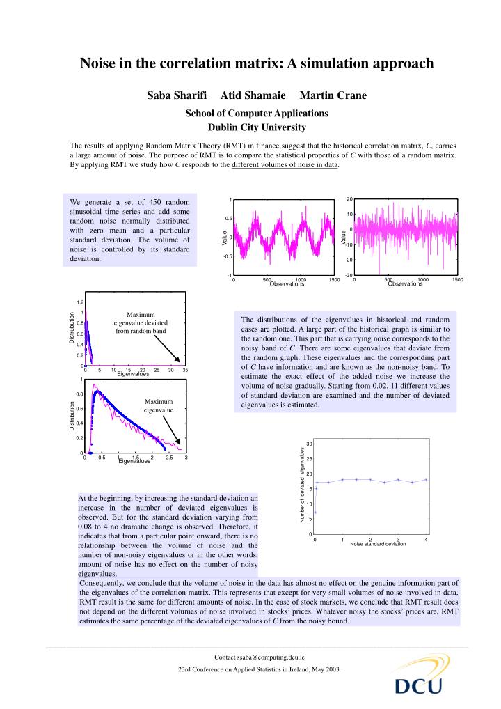
1. 1 20 10 0.5 0 0 Value Value -10 -0.5 -20 -1 -30 0 500 1000 1500 0 500 1000 1500 Observations Observations 1.2 1 0.8 Distrubution 0.6 0.4 0.2 0 0 5 10 15 20 25 30 35 Eigenvalues 1 0.8 0.6 Distribution 0.4 0.2 30 0 0 0.5 1 1.5 2 2.5 3 25 Eigenvalues eigenvalues 20 deviated 15 10 Number of 5 0 0 1 2 3 4 Noise standard deviation Noise in the correlation matrix: A simulation approach Saba Sharifi Atid Shamaie Martin Crane School of Computer Applications Dublin City University The results of applying Random Matrix Theory (RMT) in finance suggest that the historical correlation matrix, C, carries a large amount of noise. The purpose of RMT is to compare the statistical properties of C with those of a random matrix. By applying RMT we study how C responds to the different volumes of noise in data. We generate a set of 450 random sinusoidal time series and add some random noise normally distributed with zero mean and a particular standard deviation. The volume of noise is controlled by its standard deviation. Maximum eigenvalue deviated from random band The distributions of the eigenvalues in historical and random cases are plotted. A large part of the historical graph is similar to the random one. This part that is carrying noise corresponds to the noisy band of C. There are some eigenvalues that deviate from the random graph. These eigenvalues and the corresponding part of C have information and are known as the non-noisy band. To estimate the exact effect of the added noise we increase the volume of noise gradually. Starting from 0.02, 11 different values of standard deviation are examined and the number of deviated eigenvalues is estimated. Maximum eigenvalue At the beginning, by increasing the standard deviation an increase in the number of deviated eigenvalues is observed. But for the standard deviation varying from 0.08 to 4 no dramatic change is observed. Therefore, it indicates that from a particular point onward, there is no relationship between the volumeof noise and the number of non-noisy eigenvalues or in the other words, amount of noise has no effect on the number of noisy eigenvalues. Consequently, we conclude that the volume of noise in the data has almost no effect on the genuine information part of the eigenvalues of the correlation matrix. This represents that except for very small volumes of noise involved in data, RMT result is the same for different amounts of noise. In the case of stock markets, we conclude that RMT result does not depend on the different volumes of noise involved in stocks’ prices. Whatever noisy the stocks’ prices are, RMT estimates the same percentage of the deviated eigenvalues of C from the noisy bound. _____________________________________________________________________________________________________________________________ Contact ssaba@computing.dcu.ie 23rd Conference on Applied Statistics in Ireland, May 2003.