Download
1 / 91
910 likes | 989 Views
Checking Validity of Quantifier-Free Formulas in Combinations of First-Order Theories. Clark W. Barrett Ph.D. Dissertation Defense. Department of Computer Science Stanford University August 2001. The Problem: First-Order Logic.

E N D
Checking Validity of Quantifier-Free Formulas in Combinations of First-Order Theories Clark W. Barrett Ph.D. Dissertation Defense Department of Computer Science Stanford University August 2001
The Problem: First-Order Logic • First-Order Logic is a mathematical system for making precise statements. • Statements in first-order logic are made up of the following pieces: • Variablesx, y • Constants0, John, • Functionsf (x ), x + y • Predicatesp (x ), x>y, x=y • Boolean connectives, , , • Quantifiers, • Example: “Every rectangle is a square” x. (Rectangle (x )Square(x))
The Problem: First-Order Theories • A first-order theory is a set of first-order statements about a related set of constants, functions, and predicates. • A theory of arithmetic might include the following statements about 0 and +: x. ( x+ 0 =x ) x,y. (x + y = y + x )
The Problem: Validity Valid Valid Valid Invalid • An expression is valid if every possible way of interpreting it results in a true statement. x =x p(x ) p(x ) x=y f (x ) =f (y ) f (x ) =f (y ) x=y • An expression is valid in atheory if every possible way of interpreting it in that theory results in a true statement. x 0 • An expression is valid in atheory if every possible way of interpreting it in that theory results in a true statement. x 0Invalid in the theory of real arithmetic • An expression is valid in atheory if every possible way of interpreting it in that theory results in a true statement. x 0Valid in positive real arithmetic
The Problem: Validity Checking • Suppose T is a first-order theory and is a first-order formula • We write T =as an abbreviation for “ is valid in T” • A classical result in Computer Science states that in general, the question of whether T = is undecidable. • It is impossible to write a program that can always figure out whether T = • However, given appropriate restrictions on T and , a program can automatically decide T = • We consider theories Tsuch that T = is decidable when is quantifier-free.
Motivation • Many interesting and practical problems can be solved by checking the validity of a formula in some theory. • As evidence of this claim, consider the following widely-used tools tools which include decision procedures for checking validity • PVS [Owre et al. ‘92] • STeP [Manna et al. ‘96, Bjørner ‘99] • ESC [Detlefs et al. ‘98] • Mona [Klarlund and Møller ‘98] • SVC [Barrett et al. ‘96]
The SVC Story • Roots in processor verification • [Burch and Dill ‘94] • [Jones et al. ‘95] • Internal use at Stanford • Symbolic simulation [Su et al. ‘98] • Software specification checking [Park et al. ‘98] • Infinite-state model checking [Das and Dill ‘01] • External use since public release in 1998 • Model Checking [Boppana et al. ‘99] • Theorem prover proof assistance [Heilmann ‘99] • Integration into programming languages [Day et al. ‘99] • Many others
The SVC Story • Despite its success, SVC has many limitations • Gaps in theoretical understanding • Outgrown its original software architecture • Unnecessarily slow performance in some cases • This thesis is the result of ongoing efforts to address these limitations. • New contributions to underlying theory • A flexible and efficient implementation • Techniques for faster and more robust performance
Outline • Validity Checking Overview • The Problem • Motivation • The SVC Story • Top-Level Algorithm • Methods for Combining Theories • Implementation • Adapting Techniques from Propositional Satisfiability • Contributions and Conclusions
true y > x x = y false y > x x = y true y > x x = y Top-Level Algorithm • Consider the following formula in the theory of arithmetic x > y y > x x = y • Step 1: Choose an atomic formula • Step 2: Consider two cases: • Replace the atomic formula with true • Replace the atomic formula is with false • Step 3: Simplify
true x = y true false Top-Level Algorithm • Consider the following formula in the theory of arithmetic x > y y > x x = y true y > x x = y false y > x x = y true y > x x = y x y y x x y This formula is unsatisfiable
Validity Checking Overview • A literalis an atomic formula or its negation • The validity checker is built on top of a core decision procedure for satisfiability in T of a set of literals. • The method for checking satisfiability will vary greatly depending on the theory in question • The most powerful technique for producing a satisfiability procedure is by combiningother satisfiability procedures
Outline • Validity Checking Overview • Methods for Combining Theories • The Problem • Shostak’s Method • The Nelson-Oppen Method • A Combined Method • Implementation • Adapting Techniques from Propositional Satisfiability • Contributions and Conclusions
The Problem • Consider the following theories: • Real linear arithmetic: +,-,0,1,…, • Arrays:s[i], update(s,i,v) • Uninterpreted functions and predicates: f (x ), p(x ),… • And the following set of literals in the combined theory: p (y) s= update (t, i, 0 ) x-y-z=0 z+s[i] = f (x-y) p (x- f (f (z) ) ) • Consider the following theories: • Real linear arithmetic: +,-,0,1,…, • Arrays:s[i], update(s,i,v) • Uninterpreted functions and predicates: f (x ), p(x ),… • And the following set of literals in the combined theory: p (y ) s = update (t, i, 0 ) x - y - z =0 z + s[i ] = f (x - y ) p (x - f (f (z ) ) ) • Consider the following theories: • Real linear arithmetic: +,-,0,1,…, • Arrays:s[i], update(s,i,v) • Uninterpreted functions and predicates: f (x ), p(x ),… • And the following set of literals in the combined theory: p (y ) s =update (t, i, 0 ) x - y - z =0 z + s[i ]= f (x - y ) p (x - f (f (z ) ) ) • Consider the following theories: • Real linear arithmetic: +,-,0,1,…, • Arrays:s[i], update(s,i,v) • Uninterpreted functions and predicates: f (x ), p(x ),… • And the following set of literals in the combined theory: p(y ) s = update (t, i, 0 ) x - y - z =0 z + s[i ] =f (x - y ) p(x -f (f (z ) ) ) • Consider the following theories: • Real linear arithmetic: +,-,0,1,…, • Arrays:s[i], update(s,i,v) • Uninterpreted functions and predicates: f (x ), p(x ),… • And the following set of literals in the combined theory: p (y ) s = update (t, i, 0 ) x - y - z =0 z + s[i ] = f (x - y ) p (x - f (f (z ) ) ) • Question: Given a method to decide satisfiability of literals in each theory, how do we decide the satisfiability of literals in the combined theory? • Two main approaches, each with advantages and disadvantages • Shostak [Shostak ‘84] • Nelson-Oppen [Nelson and Oppen ‘79]
Shostak’s Method • Has formed an ongoing strand of research • Originally published in 1984 [Shostak ‘84] • Several clarifying papers since then • [Cyrluk et al. ‘96] • [Ruess and Shankar ‘01] • Used in several automated deduction systems • PVS, STeP, SVC • Unfortunately, remains difficult to understand • Details are nonintuitive • Simple proof of correctness has been especially elusive • Contribution: A new presentation of a key subset of Shostak’s original algorithm.
Shostak’s Method: Canonizer • There are two main components in a Shostak satisfiability procedure: the canonizerand the solver. • The canonizer rewrites terms into a unique form • T=a = b canon (a ) =canon (b ) • Example: canonizer for linear arithmetic • Combines like terms • canon (x + x ) = 2x • Imposes an ordering on the variables • canon (y + x ) =x + y
Shostak’s Method: Solver • A set of equations Eis said to be in solved form if the left-hand side of each equation is a variable which appears only once in E in solved formnot in solved form x = y + z x = y + z w = z - a w = z + x v =3y + b 2v =3y+b • S means replace each left-hand side variable occurring in S with its corresponding right-hand side E (w + x + y + z ) =z - a +y +z + y + z
Shostak’s Method: Solver • The solvertransforms an equation into an equisatisfiable set of equations in solved form • If T=a b , then solve (a = b ) ={ false } • Otherwise: • solve (a = b ) =a set of equations E in solved form • T=(a = b x.E ) • x is a set of fresh variables appearing in E, but not in a or b. • Example: solver for real linear arithmetic • solve (x - y - z =0 ) = { x = y + z } • solve (x + 1 =x -1 ) = { false }
The Simplified Algorithm • Given a set of equations and disequations • Step 1: Use the solver to convert into an equisatisfiable set of equations E in solved form • Use a generalization of Gaussian elimination with back substitution
Choose matrix row E -x -3y +2z =-1 x -y -6z = 1 2x + y -10z= 3 The Simplified Algorithm • Given a set of equations and disequations • Step 1: Use the solver to convert into an equisatisfiable set of equations E in solved form • Select an equation from • Apply E as a substitution to • Solve to get E’ • Apply E’ as a substitution to E • Add E’ to E
Apply previous rows E -x -3y +2z =-1 x -y -6z = 1 2x + y -10z= 3 The Simplified Algorithm • Given a set of equations and disequations • Step 1: Use the solver to convert into an equisatisfiable set of equations E in solved form • Select an equation from • Apply E as a substitution to • Solve to get E’ • Apply E’ as a substitution to E • Add E’ to E Choose matrix row
Apply to previous rows E The Simplified Algorithm • Given a set of equations and disequations • Step 1: Use the solver to convert into an equisatisfiable set of equations E in solved form • Select an equation from • Apply E as a substitution to • Solve to get E’ • Apply E’ as a substitution to E • Add E’ to E Choose matrix row Apply previous rows Make pivot 1 x =-3y +2z +1 x -y -6z = 1 2x + y -10z= 3
E The Simplified Algorithm • Given a set of equations and disequations • Step 1: Use the solver to convert into an equisatisfiable set of equations E in solved form • Select an equation from • Apply E as a substitution to • Solve to get E’ • Apply E’ as a substitution to E • Add E’ to E Choose matrix row Apply previous rows Make pivot 1 Apply to previous rows x -y -6z = 1 2x + y -10z= 3 x =-3y +2z +1
E The Simplified Algorithm • Given a set of equations and disequations • Step 1: Use the solver to convert into an equisatisfiable set of equations E in solved form • Select an equation from • Apply E as a substitution to • Solve to get E’ • Apply E’ as a substitution to E • Add E’ to E Choose matrix row Apply previous rows Make pivot 1 Apply to previous rows x =-3y +2z +1 -3y +2z +1-y -6z =1 2x + y -10z= 3
E The Simplified Algorithm • Given a set of equations and disequations • Step 1: Use the solver to convert into an equisatisfiable set of equations E in solved form • Select an equation from • Apply E as a substitution to • Solve to get E’ • Apply E’ as a substitution to E • Add E’ to E Choose matrix row Apply previous rows Make pivot 1 Apply to previous rows x =-3y +2z +1 y =-z 2x + y -10z= 3
E The Simplified Algorithm • Given a set of equations and disequations • Step 1: Use the solver to convert into an equisatisfiable set of equations E in solved form • Select an equation from • Apply E as a substitution to • Solve to get E’ • Apply E’ as a substitution to E • Add E’ to E Choose matrix row Apply previous rows Make pivot 1 Apply to previous rows x =-3(-z)+2z +1 y =-z 2x + y -10z= 3
E The Simplified Algorithm • Given a set of equations and disequations • Step 1: Use the solver to convert into an equisatisfiable set of equations E in solved form • Select an equation from • Apply E as a substitution to • Solve to get E’ • Apply E’ as a substitution to E • Add E’ to E Choose matrix row Apply previous rows Make pivot 1 Apply to previous rows 2x + y -10z= 3 x =5z +1 y =-z
E The Simplified Algorithm • Given a set of equations and disequations • Step 1: Use the solver to convert into an equisatisfiable set of equations E in solved form • Select an equation from • Apply E as a substitution to • Solve to get E’ • Apply E’ as a substitution to E • Add E’ to E Choose matrix row Apply previous rows Make pivot 1 Apply to previous rows x =5z +1 y =-z 2(5z +1)+(-z )-10z=3
E The Simplified Algorithm • Given a set of equations and disequations • Step 1: Use the solver to convert into an equisatisfiable set of equations E in solved form • Select an equation from • Apply E as a substitution to • Solve to get E’ • Apply E’ as a substitution to E • Add E’ to E Choose matrix row Apply previous rows Make pivot 1 Apply to previous rows z =-1 x =5z +1 y =-z
E The Simplified Algorithm • Given a set of equations and disequations • Step 1: Use the solver to convert into an equisatisfiable set of equations E in solved form • Select an equation from • Apply E as a substitution to • Solve to get E’ • Apply E’ as a substitution to E • Add E’ to E Choose matrix row Apply previous rows Make pivot 1 Apply to previous rows z =-1 x =5(-1)+1 y =-(-1)
E The Simplified Algorithm • Given a set of equations and disequations • Step 1: Use the solver to convert into an equisatisfiable set of equations E in solved form • Select an equation from • Apply E as a substitution to • Solve to get E’ • Apply E’ as a substitution to E • Add E’ to E Choose matrix row Apply previous rows Make pivot 1 Apply to previous rows x =-4 y =1 z =-1
E 4242 2(1)-10(-4)6(-1-2(-4)) 2y -10x 6(z -2x) The Simplified Algorithm • Given a set of equations and disequations • Step 1: Use the solver to convert into an equisatisfiable set of equations E in solved form • Step 2: Use this set of equations together with the canonizer to check if any disequality is violated • For each a b • Check if canon (E (a ) ) =canon (E (b ) ) x =-4 y =1 z =-1
E 1- 4y x - z 4z +14z +1 1-4(-z)(5z +1)-z The Simplified Algorithm • Given a set of equations and disequations • Step 1: Use the solver to convert into an equisatisfiable set of equations E in solved form • Step 2: Use this set of equations together with the canonizer to check if any disequality is violated • For each a b • Check if canon (E (a ) ) =canon (E (b ) ) x =5z +1 y =-z
The Simplified Algorithm • Given a set of equations and disequations • Step 1: Use the solver to convert into an equisatisfiable set of equations E in solved form • Step 2: Use this set of equations together with the canonizer to check if any disequality is violated • For each a b • Check if canon (E (a ) ) =canon (E (b ) ) • Technical detail: • If there is more than one disequality, the theory must be convex
Shostak’s Method: Combining Theories • In what sense is this algorithm a method for combining theories? • Two Shostak theories T1 and T2 can often be combined to form a new Shostak theory T =T2T2 • Compose canonizers: canon=canon1ocanon2 • Often, solvers can also be combined • Treat terms from other theory as variables • Repeatedly apply solvers from each theory until resulting set of equations is in solved form
Shostak’s Method: Contributions • Shostak’s original algorithm is much more complicated because it includes a decision procedure for the theory of pure equality with uninterpreted functions • Why is the simplified version a contribution? • Can be applied directly to produce decision procedures, even combinations of decision procedures • Much easier to understand and prove correct • Provides intuition for understanding the original algorithm • Provides the foundation for a generalization of the original Shostak method based on a variation of Nelson-Oppen
Nelson-Oppen • Developed for the Stanford Pascal Verifier • [Nelson and Oppen ‘79] • [Nelson ‘80, Oppen ‘80] • Tinelli and Harandi discovered a new (simpler) proof and an important optimization • [Tinelli and Harandi ‘96] • Used in real systems • ESC • EHDM [von Henke et al. ‘88] • Vampyre [http://www-cad.eecs.berkeley.edu/~rupak/Vampyre]
Nelson-Oppen • Unlike Shostak, Nelson-Oppen does not impose a specific strategy on individual theories • Instead of a solver and canonizer, • Each theory provides a complete satisfiability procedure • Technical detail: Each theory must be stably infinite • There are two phases in the version of Nelson-Oppen presented by Tinelli and Harandi • Purification phase • Check phase
Nelson-Oppen: Purification Phase • Transform a set of literals in a combined theory to an equisatisfiable set of literals such that each literal is pure : • A pure literalcontains symbols from only a single theory • Consider again the following set of literals in a combined theory of arithmetic, arrays, and uninterpreted functions p(y ) s =update (t, i, 0 ) x - y - z =0 z + s[i ]=f(x - y ) p(x -f (f (z ) ) ) j =0
Nelson-Oppen: Purification Phase • Transform a set of literals in a combined theory to an equisatisfiable set of literals such that each literal is pure : • A pure literalcontains symbols from only a single theory • Consider again the following set of literals in a combined theory of arithmetic, arrays, and uninterpreted functions p(y ) s =update (t, i, j ) x - y - z = j z + s[i ]=f(x - y ) p(x -f (f (z ) ) ) j =0 j =0 k = s[i ]
Nelson-Oppen: Purification Phase • Transform a set of literals in a combined theory to an equisatisfiable set of literals such that each literal is pure : • A pure literalcontains symbols from only a single theory • Consider again the following set of literals in a combined theory of arithmetic, arrays, and uninterpreted functions p(y ) s =update (t, i, j ) x - y - z = j z + k=f(x - y ) p(x -f (f (z ) ) ) j =0 k = s[i ] j =0 k = s[i ] l = x - y m = z + k
Nelson-Oppen: Purification Phase • Transform a set of literals in a combined theory to an equisatisfiable set of literals such that each literal is pure : • A pure literalcontains symbols from only a single theory • Consider again the following set of literals in a combined theory of arithmetic, arrays, and uninterpreted functions p(y ) s =update (t, i, j ) l - z = j m=f(l ) p(x -f (f (z ) ) ) j =0 k = s[i ] l = x - y m = z + k
Nelson-Oppen: Purification Phase • Transform a set of literals in a combined theory to an equisatisfiable set of literals such that each literal is pure : • A pure literalcontains symbols from only a single theory • Consider again the following set of literals in a combined theory of arithmetic, arrays, and uninterpreted functions p(y ) s =update (t, i, j ) l - z = j m=f(l ) p(v ) j =0 k = s[i ] l = x - y m = z + k n =f (f (z ) ) ) v = x - n
Nelson-Oppen: Purification Phase • Transform a set of literals in a combined theory to an equisatisfiable set of literals such that each literal is pure : • A pure literalcontains symbols from only a single theory • Consider again the following set of literals in a combined theory of arithmetic, arrays, and uninterpreted functions p(y ) m=f(l ) p(v ) n =f (f (z ) ) ) s =update (t, i, j ) k = s[i ] l - z = j j =0 l = x - y m = z + k v = x - n
p(y ) m=f(l ) p(v ) n =f (f (z ) ) ) s =update (t, i, j ) k = s[i ] l - z = j j =0 l = x - y m = z + k v = x - n Nelson-Oppen: Check Phase Definitions • Shared variables are variables that appear in literals from more than one theory • Shared: l, z, j, y, m, k, v, n • Unshared: x, s, t, i • An arrangementof a set is a set of equalities that partitions the set into equivalence classes • Suppose S ={ a , b , c } • Some arrangements of S • { a b , a c , bc } { { a } , { b } , { c } } • { a = b , a c , bc } { { a , b } , { c } } • { a = b , a = c , b=c } { { a , b , c } }
Nelson-Oppen: Check Phase • Choose an arrangementAof the shared variables • For each theory, check if the set of literals pure in that theory together with the arrangement A is satisfiable • If an arrangement exists that is compatible with each set of literals, then the original set of literals is satisfiable in the combined theory Arithmetic l - z = j j =0 l = x - y m = z + k v = x - n Arrays s =update (t, i, j ) k = s[i ] Uninterpreted p(y ) m=f(l ) p(v ) n =f (f (z ) ) ) A (l, z, j, y, m, k, v, n )
Arithmetic x - y - z =0 z + s[i ]=f(x - y ) Arrays s =update (t, i, 0 ) Uninterpreted p(y ) p(x -f (f (z ) ) ) Nelson-Oppen: A Variation • Contribution : A Variation of Nelson-Oppen • The purification phase can be eliminated • Instead, simply partition the formulas according to the outer-most symbol p(y ) s =update (t, i, 0 ) x - y - z =0 z + s[i ]=f(x - y ) p(x -f (f (z ) ) )
Arithmetic x - y - z =0 z + s[i ]=f(x - y ) Arrays s =update (t, i, 0 ) Uninterpreted p(y ) p(x -f (f (z ) ) ) A (s[i ], x - y, f(x - y ), 0,y, z, f (f (z ) ), x -f (f (z ) ) ) Nelson-Oppen: A Variation • Contribution : A Variation of Nelson-Oppen • The purification phase can be eliminated • Instead, simply partition the formulas according to the outer-most symbol • Choose an arrangement A of the shared terms which appear in a term or formula belonging to another theory • For each theory, check if the set of literals assigned to that theory together with the arrangement is satisfiable • Terms with foreign symbols are treated as variables
Nelson-Oppen: A Variation • Contribution : A Variation of Nelson-Oppen • The purification phase can be eliminated • Instead, simply partition the formulas according to the outer-most symbol • Choose an arrangement A of the shared terms which appear in a term or formula belonging to another theory • For each theory, check if the set of literals assigned to that theory together with the arrangement is satisfiable • Terms with foreign symbols are treated as variables • Contributions of this variation • Fewer formulas given to each theory • Easier to implement • Easier to combine with Shostak
Combining Shostak and Nelson-Oppen • Theory requirements • Shostak requires convexity • Nelson-Oppen requires stable-infiniteness • Contribution : The following theorem relates the two Every convex first-order theory with no trivial models is stably-infinite • The proof is based on first-order compactness • Note: if a convex theory does admit trivial models, it can usually be modified to include the non-triviality axiom: x,y. x y