METHOD

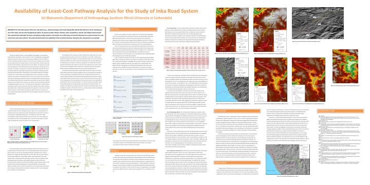
1. Zone 1 (Cañar-Azuay) Due to the unknown datum and the poor resolution of the scanned map, there is a high probability that the locations of the digitized polyline and point features (roads and sites) are not very accurate. Given this fact, nonetheless, the northern half of the shared path from Ingapirca to Achupallas to the north is relatively approximate to the preserved/reconstructed road segments, while the southern half follows a completely different route from the preserved/reconstructed (Figure 4). As clearly seen here, the calculated prefers traveling on the valley floor to reduce the cost, while the preserved/reconstructed tends to choose the shortest route even at the expense of additional energy expenditure. [ABSTRACT] The inferred purposes of the Inca road system (e.g., relaying messages and transporting goods) indicate that minimum cost for traveling was one of the major concerns when designing the system. As previous studies indicate, however, other sociopolitical, cultural, and religious factors should have operated intertwiningly. The least-cost pathway analysis based on anisotropic cost surface helps to inversely delineate non-economic factors for road construction and route selection. This study will demonstrate the availability of this analytical technique, taking the Inka road system as an example. METHOD The data source available for this study is quite limited. The famed Proyecto Qhapaq Ñan Cusco has not yet published any comprehensive map of the Inka Road (Amado Gonzales 2005; Ugarte Vega Centeno 2005). As of the moment, the only maps that can be scanned and integrated into GIS overlay are those recorded by Hyslop (1984) from the late 70’s to the early 80’s. Out of the 12 zones that Hyslop recorded, the first three zones (Cañar-Azuay, Lambayeque-Moche, and Cajamarca-Huamachuco) were selected due to the time constraints (Figure 2). There is no description in either maps or texts about the map datum by which each of the maps was projected. Taking into account that the original maps based on which Hyslop’s maps were created were all produced during the 60’s to the 70’s in Ecuador or Peru, I speculate that the Provisional South American Datum 1956 (PSAD56) was used. Both preserved and reconstructed segments of the road system were scanned, georeferenced, and digitized together with archaeological sites and modern-day populations. In order to create the anisotropic cost surface, sets of free Digital Elevation Models (SRTM, Degree Tiles) of relatively low resolution were utilized. For the large size of the study areas (e.g., Zone 1 of approximately 4,000 km² or 400,000 hectares), the 90-m resolution would be quite adequate. Subsets including the study areas were clipped off of a combined image of the adjacent DEM tiles. Patching data loss and defining UTM coordinates for the subsets were conducted by means of 3DEM, free software available online. The procedures to create an anisotropic cost surface are summarized below in the form of expressions used in ArcGIS Raster Calculator: Figure 6: A Three-Dimensional View of the Calculated Paths for Zone 1 INTRODUCTION HYPOTHESIS Figure 4: The Least-Cost Paths for Zone 1 (Reproduced from Hyslop 1984:20, fig. 2.1) Figure 5: Inter-Site Paths for Zone 1 (Reproduced from Hyslop 1984:20, fig. 2.1) An escapeway from this cul-de-sac is to further refine the cost surface raster so as to more accurately delineate the traveler’s concern for cost-efficiency. A recent shift in emphasis from isotropic to anisotropic costs enables us to represent different modes of travel across slope more precisely and faithfully to the reality. Anisotropic modeling takes into account the difference in cost depending upon the direction of travel (e.g., perpendicular to or parallel with the aspect? upslope or downslope?), while isotropic one fails to do so and simply assumes a certain amount of cost for each cell regardless of the travel direction. Consequently, the former may provide different routes for outward and homeward journeys, whereas the latter does not. A recent field experiment directed by Yasuhisa Kondo (University of Tokyo) in Kozu Island, Japan revealed that the least-cost path calculated by means of an anisotropic, accumulated cost surface is by and large in close alignment with the route selected by travelers who favor the ”ease of traveling. In likewise, if the calculated path prioritizing the minimum cost for traveling can adequately capture a possible, economic concern of those who built and traveled a road, in theory, the gaps between the calculated path and the preserved road have to be explained from something other than an economic perspective. As a result, by focusing on those gaps, I suspect that it would be possible to inversely shed light on the unknown, non-economic factors. This hypothesis is tested below by calculating some least-cost paths for the Inka Road System, which is thought to have been used for both economic (e.g., relaying messages and transporting goods) and symbolic functions (e.g., representing ceque lines). The least-cost pathway analysis, normally equipped in GIS packages, is an oft-employed analytical tool for simulating the “most economical” route for traveling between archaeological settlements and natural resources and. As Conolly and Lake (2006:252) note, this method has often been employed to predict the location of unpreserved ancient transport routes. As long as we keep using it solely for this purpose, however, we will never be able to link the results to the true picture of the prehistoric road construction and route selection. This means that we cannot assess the effectiveness of the method and may end up with wasting our limited resources just for a guess. For example, it was because of its empirical modeling and testing with reference to the actual distribution of archaeological settlements that the predictive modeling was widely accepted and eventually became a defining feature of archaeological application of GIS-aided analytical tools. In order for the least-cost pathway analysis to earn a reputation as a reliable method to solve authentic archaeological problems, the accuracy and precision of the modeling need to be refined through a comparative study of the calculated and the preserved routes (e.g., Krist and Brown 1994). Furthermore, because the route selection may vary not only for different purposes, but also in different times and areas, we should not assume an all-purpose model that is thoughtlessly applicable to any case. In this regard, the Inka Road System is an ideal subject of this analysis, because it covers an immense area of diverse regional cultures and environmental characteristics and is, if partially, still preserved either on the ground or in the record. As the first step of my long-term research effort to elucidate interregional interactions in the Andes, this study is aimed at examining the availability of the least-cost pathway analysis for the study of the Inka Road System. Availability of Least-Cost Pathway Analysis for the Study of Inka Road System Go Matsumoto (Department of Anthropology, Southern Illinois University at Carbondale) Table 2: Comparison of total length, slope degree, travel cost and time for the ten paths in Zone 1 In Table 2, the calculated paths are longer than the preserved/reconstructed road segments, because the employed model always attempts to avoid steeper slopes that take more time to travel. It is paradoxical, however, that this approach may lead to increase the travel time as in the calculated paths 3 and 4. This is probably because the model cannot examine the topography as a whole, but only considers “one step forward,” that is, the immediate eight cells that surround the cell in question. Consequently, depending upon the topography and the locations of origin and destination(s), an unrealistically long path may be provided. Nevertheless, the calculated paths 1 and 2 successfully reduced slope degree, travel cost, and travel time. On the other hand, the Inka Road in some places seems to have been designed to link adjacent sites with the shortest paths rather than to reduce the travel cost right in front. It is likely that priority was placed on traveling through those sites in order. This could be for relaying messages by chaski or for expressing some symbolic importance just like the concept of “roads through time” that represent symbolic links between religious features from different time periods (Adler 1994; Fowler and Stein 1992). Regarding the transportation of goods by caravans of camelids, however, the maximum slope of 42.04˚ may be the greatest obstacle. The road system should have been critical in this area for the military campaigns to conquest the Cañari and the Puruhua to the north. It is undeniable that there may have been another road that was used for cargo shipment but is yet to be found along the calculated path. Zone 2 (Lambayeque-Moche) The northward and northward least-cost paths in Zone 2 were calculated by means of the accumulated cost surface that was generated from a specially prepared DEM. Since SRTM Degree Tiles (DEMs) involve elevation values not only for the terrain surface, but also for the surface of the sea, the latter need to be excluded (or replaced with unrealistically high cost values) in order to gain only an overland path. Otherwise, as shown in Path 3 in Figure 7, water route may be given as the least-cost path. This is very noteworthy because Path 3 indicates the possibility that the coastal population may have sailed in the sea for some economic functions such as long-distance trade along the coast. Needless to say, the surface conditions of the sea have to be carefully modeled by taking into account tide and currents. Most of the currently available models for the least-cost pathway analysis view terrain slope and aspect as a primary cost of traveling; therefore, the calculated path always circumnavigates hills and mountain ridges. Unexceptional is the coastal area where the slope is trivial. The preserved road segments on the coast, however, seems to persistently draw a straight line, even in the rugged area (between Tambo Real and Canteras in Figure 7) allowing for additional energy expenditure. For the travel on the coast, viewshed rather than ease of traveling may have been prioritized. Thus, two notable gaps between the calculated paths and the preserved/ reconstructed road segments were observed: one between Tambo Real and Canteras and the other between Desert Site to Chinquitoy Viejo. Zone 3 (Cajamarca-Huamachuco) Like the previous zones described above, the calculated paths to different destinations, Paths 1 and 2, share a single path that is parallel to the preserved/reconstructed road segments and is in complete alignment with the valley floors of Cajamarca and Condebamba Rivers (Figure 8).The unique paths branching off into the destinations are very approximate to the preserved road segment in the northern half of Paths 1 and 2, while those in the southern half show significant gaps. Two additional inter-site paths were also calculated in order to clarify the reason for these gaps: Path 3 between Baños del Inka and Namora and Path 4 between Ichocan and Cauday (Figure 9). Path 3 follows a totally different path from the one reconstructed by Hyslop (1984) and is more approximate to the modern-day road connecting Cajamarca and Namora. I suspect that the reconstructed segment may not have exited and that another path similar to the modern-day road linked Cajamarca and the preserved segment near Namora. Likewise, Path 4 does not cross the Crisnejas River as the preserved road does, but rather takes a route similar to the modern-day road. Figure 10: A Three-Dimensional View of the Calculated Paths for Zone 3 a.[bklink2] b.[flowdir] c. [diff2] ([diff3]) d. Five types of movement Figure 3: The creation of an anisotropic cost surface. LEAST-COST PATHWAY ANALYSIS Figure 9: Inter-Site Paths for Zone 3 (Reproduced from Hyslop 1984:57, fig. 4.1) Figure 7: The Least-Cost Paths for Zone 2 (Reproduced from Hyslop 1984:38, fig. 3.1) Figure 8: The Least-Cost Paths for Zone 3 (Reproduced from Hyslop 1984:57, fig. 4.1) In the least-cost pathway analysis, the route is calculated based on the accumulated cost surface that models the cost of traveling from a given origin to one or more destinations. As moving over the cost-of-traveling raster map to each destination, the cost value in each cell is accumulated by a spreading function (Figure 1). The resultant cost raster is then called accumulated cost surface and used to find the least-cost route over it. For the creation of an accumulated cost surface, most GIS packages require a minimum of three dataset: (1) traffic origin; (2) destination(s); and (3) cost surface (or cost-of-traveling) raster. only for the study of Inka Road System, but also for the interregional interactions in the Andes. As the next step of this long-term research, priority will be placed on: (1) reexamination and refinement of the “one-step-forward” model; (2) improvement of data quality; and (3) establishment of an additional model and formula to predict water routes. Furthermore, as I noted elsewhere (Matsumoto 2005, in press), the improved model also needs to involve postprocessualistic concerns for subjectivity, for example, sense of distance. Commonly, adults walk longer and faster than children, and a caravan of men and animals travels faster across a wider range of area when they do so without a heavy burden. Furthermore, the perceived distance may not necessarily be commensurate with the amount of time that they actually spend. It may also vary depending on certain factors such as the type of activity (e.g., messaging, pilgrimage, expedition, trade, farming, fishing, hunting, and so forth). This concept of perceived distance would help us to quantify the perceived landscape. It will allow for a refinement of the conventional ideal models such as region segmentation (e.g., central place theory and Thiessen polygons) and optimum path analyses as well. By sorting the perceived distance into different categories, one can generate a series of cost surfaces different in range and apply them to create the sub-models that are more faithful to the past landscape. In order to achieve this, the reference to the ethnohistorical and ethnographic records will be essential. DISCUSSIONS REFERENCES CITED As indicated above, there is a slight chance that new road segments may be found along the calculated paths, especially along those in Zones 1 and 3. In order to reliably detect the presence of those unseen road segments, improvement of data quality and ground-truth checking of the already found segments by means of Global Positioning System (GPS) are essential. The study areas are truly immense. Not all preserved roads could have been found by Hyslop. In fact, for Zone 1, Fresco (2004) recently reported as “secondary roads” some new paths that had not been recorded by Hyslop: three stretching east, west, and southwest from Tomebamba, one branching off of the artery near Deleg and heading for the northeast, and another stretching northwest from Ingapirca. This study not only demonstrates that the least-cost pathway analysis is a useful analytical tool, but also highlights some of the limitations and weaknesses of the current model and calculation formula. First of all, the model cannot view the topography as a whole, but only examines the travel cost in the immediate eight cells that surround the cell in question. As a result, the resulting path may be unrealistically long, circumnavigating costly up and downslopes. Secondly, the least-cost path may not be unique. Kondo (2007) demonstrates that different GIS packages provide different least-cost paths. In this study, none of the calculated paths is in perfect alignment with the preserved/reconstructed road segments. As Kondo (in press) argues, adopting the concept of “least-cost corridor,” we may have to consider the different paths within a corridor as the same route. Thirdly, because the method always attempts to find the least-cost path even in the area where the slope is trivial, the resulting route may make an unnecessary detour. Thus, the current model would be more suitable for the study of movement in the highlands and the interregional interactions between the highlands and the coast (Figure 11). Adler, Michael 1994 Population aggregation and the Anasazi social landscape: A view from the Four Corners. In The Ancient Southwestern Community, edited by W. H. Wills and R. D. Leonard, pp. 85-102. University of New Mexico Press, Albuquerque. Amado Gonzales, D. D. 2005 Sistema vial andino en el valle de Cusco. Qhapaq-Ñan del Tawantinsuyu 1:7-23. Bell, T. and G. Lock 2000 Topographic and Cultural Influences on Walking the Ridgeway in Later Prehistoric Times. In Beyond the Map: Archaeology and Spatial Technologies, edited by G. Lock, pp. 85-100. IOS Press, Amsterdam. Conolly, J. and M. Lake 2006 Geographic Information Systems in Archaeology. Manuals in Archaeology. Cambridge University Press, Cambridge. Fowler, Andrew P. And John R. Stein 1992 The Anasazi Great House in space, time, and paradigm. In Anasazi Regional Organization and the Chaco System, edited by D. E. Doyel, pp. 101-122. Maxwell Museum of Anthropology Anthropological Papers No. 5. University of New Mexico, Albuquerque. Fresco, A. 2004 Ingañán: La red vial del imperio inca en los Andes ecuatoriales. Banco Central del Equador, Quito. Hyslop, J. 1984 The Inka Road System. Studies in Archaeology. Academic Press, Orlando. Kantner, J. 1996 An Evaluation of Chaco Anasazi Roadways. Paper presented at the 61st Annual Meeting of the Society for American Archaeology, New Orleans, Louisiana. Kondo, Y. 2007 Rethinking GIS-based Travel Cost Modeling. Paper presented at the the 24th Semiannual Meeting of Japan Society for Archaeological Information, Keio University, Tokyo, Japan.  in press From Pathways to Corridor: Rethinking GIS-based Travel Cost Modeling. Archaeological Information 14(1). Krist, F. J. and D. G. Brown 1994 GIS Modeling of Paleo-Indian period caribou migrations and viewsheds in northern Lower Michigan. Photogrammetric Engineering and Remote Sensing 60:1129-1137. Llobera, M. 2000 Understanding Movement: A Pilot Model Towards the Sociology of Movement. In Beyond the Map: Archaeology and Spatial Technologies, edited by G. Lock, pp. 65-84. IOS Press, Amsterdam. Tobler, W. 1993 Three presentations on geographical analysis and modeling. Technical Report 93-1, National Center for Geographic Information and Analysis, University of California. Ugarte Vega Centeno, D. 2005 Prologo. Qhapaq-Ñan del Tawantinsuyu 1:5. van Leusen, P. M. 2002 Pattern to Process: Methodological Investigations into the Formation and Interpretation of Spatial Patterns in Archaeological Landscapes, Unpublished Ph.D. Dissertation, University of Groningen. Table 1: The procedures to create an anisotropic cost surface (originally coded by Yasuhisa Kondo, University of Tokyo). a. Origin and Destination b. Cost-surface c. Cumulative Cost-surface The anisotropic cost surface is then processed to generate an accumulated cost surface by means of Cost Distance function of the ArcGIS Spatial Analyst extension. Based on the resultant, accumulated cost surface, the least-cost paths are calculated. Figure 1: Finding the least-cost route by reiterating a basic spreading function over the cost-surface (Reproduced from Conolly and Lake 2006:222, fig. 10.11). The way of creating cost surface varies depending on the type of cost that you assume for the determination of accessibility. Most of the currently available models view the slope and aspect of terrain as a primary cost of traveling and attempt to quantify the cost in terms of elapsed time or energetic expenditure (Bell and Lock 2000; Tobler 1993; van Leusen 2002). As previous studies indicate (e.g., Kantner 1996), however, other sociopolitical, cultural, and religious factors could have operated intertwiningly. Under the influence of postprocessualist thinking about space and landscape, Llobera (2000) integrates the cultural influence of monuments into the energetic cost of traveling. Nonetheless, unlike the physical “frictions” that can be measured and quantified objectively, it may be quite difficult to represent those, oftentimes intangible, factors in the form of map with the same resolution and scale as those of other map layers and to sophisticate the model to a satisfactory level for many archaeologists. Here is a limitation of this analytical tool. RESULTS Setting the northernmost and southernmost sites in each zone as the traffic origins and the rest of the sites located along the preserved/reconstructed segments of the Inka Road (both Inka sites and modern-day populations) as destinations, both northward and southward routes were calculated. It was revealed that all but a few of the resulting routes share a single path and then branch off into a unique path to each destination (Figures 4, 7, and 8). Expectedly, in some areas, both gaps and close alignments between the calculated paths and the preserved/reconstructed road segments came into focus. In order to clarify the reason for the gaps between the calculated and preserved, additional inter-site routes were also calculated for Zones 1 and 3 (Figures 5 and 9). CONCLUSION Through a series of calculations of the most economical routes between given two loci, the least-cost pathway analysis proved to be a useful analytical tool, although it still leaves some weaknesses to be improved. Once these weaknesses are overcome and its availability is further validated with reference to the preserved road segments, this method will be very powerful not Figure 2: Inka Road System (Taken from Hyslop 1984) Figure 11: Inter-Artery Paths Between Zones 2 and 3