Central Limit Theorem and Introduction to Uncertainty

1. Central Limit Theorem and Introduction to Uncertainty Physics 270 – Experimental Physics

2. Standard Deviation To calculate the standard deviation for a sample of 5 (or more generally n) measurements: 1. Sum all the measurements and divide by 5 (n) to get the average or mean, . 2. Now, subtract this average from each of the 5 (n) measurements to obtain 5 "deviations." 3. Square each of these 5 (n) deviations and add them all up. 4. Divide this result by 5 (n), and take the square root.

3. Example: Width of sheets of paper

4. Standard Deviation of the Mean (Standard Error) When we report the average value of n measurements, the uncertainty we should associate with this average value is the standard deviation of the mean, often called the standard error (SE): This reflects the fact that we expect the uncertainty of the average value to get smaller when we use a larger number of measurements n.

5. Example: Width of sheets of paper

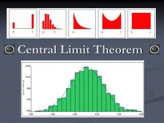
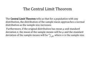
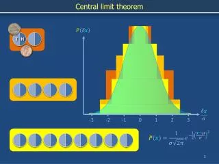
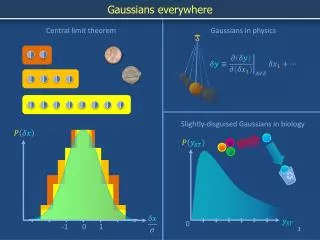
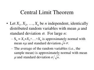
6. Central Limit Theorem The Gaussian distribution works well for any random variable because of the Central Limit Theorem. A simple description of it is… When data that are influenced by many small and unrelated random effects, it will be approximately normally distributed. Let Y1, Y2, … Ynbe an infinite sequence of independent random variables, usually from the same probability distribution function, but it could be different pdf’s.

7. Central Limit Theorem Suppose that the mean, µ, and the variance 2 are both finite. For any two numbers a and b… CLT tells us that under a wide range of circumstances the probability distribution that describes the sum of random variables tends towards a Gaussian distribution as the number of terms in the sum → ∞.

8. Example: Computer Random Numbers Random number generator gives numbers distributed uniformly in the interval [0,1] µ = 1/2 and σ2 = 1/12 Take 12 numbers, add them together, then subtract 6. You get a number that looks as if it is from a Gaussian pdf!

9. Example: Computer Random Numbers Take 12 numbers, add them together, then subtract 6…

10. Uncertainty of Measurements • Some statements are exact… • Jessica has 6 Webkinz. • 7 + 2 = 9 • All measurements have uncertainty. • “uncertainty” versus “error” • measurement = best estimate ± uncertainty • Tennis ball example Measurement = (measured value ± standard uncertainty) unit of measurement

11. Types of Errors • Random errors are statistical fluctuations (in either direction) in the measured data due to the precision limitations of the measurement device. Random errors can be evaluated through statistical analysis and can be reduced by averaging over a large number of observations. • Systematic errors are reproducible inaccuracies that are consistently in the same direction. These errors are difficult to detect and cannot be analyzed statistically. If a systematic error is identified when calibrating against a standard, the bias can be reduced by applying a correction or correction factor to compensate for the effect. Unlike random errors, systematic errors cannot be detected or reduced by increasing the number of observations.

12. Example: Mass Determination = 50 grams = 20 grams = 5 grams 70 g ≤ mass ≤ 80 g mass = 75 ± 5 g

13. Example: Mass Determination • more precise • more accurate? • ± 0.1 g • m = 74.6 ± 0.1 g • m = 74.6 ± 0.2 g • two 200 g calibration masses included 0.00 74.6

14. Textbook Values • results of one experiment • results of many experiments • National Institute Standards and Technology • http://physics.nist.gov/cuu/Constants/ • other international organizations

15. Anomalous Data • Outliers • Could be significant or insignificant. • Don’t just throw away data.