Multiple Regression

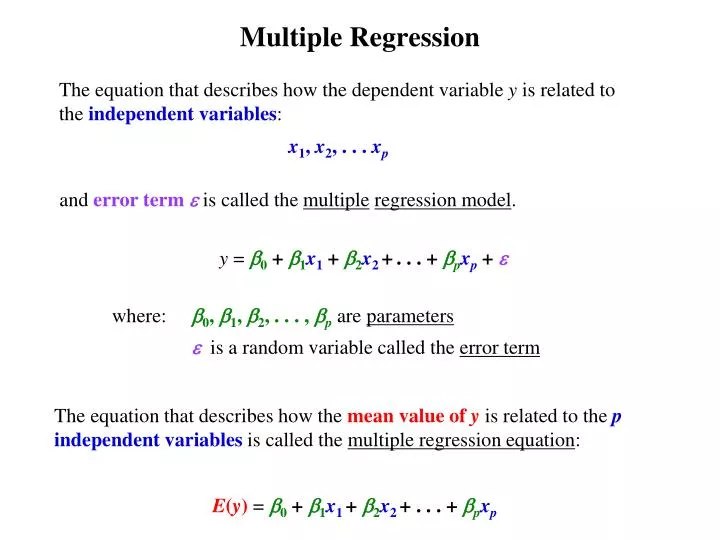
Multiple Regression • The equation that describes how the dependent variable y is related to the independent variables: x1, x2, . . . xp and error term e is called the multipleregression model. y = b0 + b1x1 + b2x2+. . . + bpxp + e where: b0, b1, b2, . . . , bp are parameters e is a random variable called the error term The equation that describes how the mean value of y is related to the p independent variables is called the multiple regression equation: E(y) = 0 + 1x1+ 2x2+ . . . + pxp

Multiple Regression A simple random sample is used to compute sample statistics b0, b1, b2, . . . , bp that are used as the point estimators of the parameters b0, b1, b2, . . . , bp The equation that describes how the predicted value of y is related to the p independent variables is called the estimated multiple regression equation: ^ y = b0 + b1x1+ b2x2+ . . . + bpxp

Specification • Formulate a research question: • How has welfare reform affected employment of low-income mothers? • Issue 1: How should welfare reform be defined? • Since we are talking about aspects of welfare reform that influence the decision to work, we include the following variables: • Welfare payments allow the head of household to work less. • tanfben3= real value (in 1983 $) of the welfare • payment to a family of 3 (x1) • The Republican lead Congress passed welfare reform twice, both of which were vetoed by President Clinton. Clinton signed it into law after the Congress passed it a third time in 1996. All states put their TANF programs in place by 2000. • 2000 = 1 if the year is 2000, 0 if it is 1994 (x2)

Specification • Formulate a research question: • How has welfare reform affected employment of low-income mothers? • Issue 1: How should welfare reform be defined?(continued) • Families receive full sanctions if the head of household fails to adhere to a state’s work requirement. • fullsanction = 1 if state adopted policy, 0 otherwise (x3) • Issue 2: How should employment be defined? • One might use the employment-population ratio of Low-Income Single Mothers (LISM):

Specification 2. Use economic theory or intuition to determine what the true regression model might look like. Use economic graphs to derive testable hypotheses: Consumption Economic theory suggests the following is not true: Ho: b1 = 0 550 U1 400 U0 300 Receiving the welfare check 55 40 Leisure increases LISM’s leisure which decreases hours worked

Specification 2. Use economic theory or intuition to determine what the true regression model might look like. Use a mathematical model to derive testable hypotheses: The solution of this problem is: Economic theory suggests the following is not true: Ho: b1 = 0

Specification 3. Compute means, standard deviations, minimums and maximums for the variables.

Specification 4. Construct scatterplots of the variables. (1994, 2000)

Specification • 5. Compute correlations for all pairs of variables. If | r | > .7 for a pair of independent variables, • multicollinearity may be a problem • Some say avoid including independent variables that are highly correlated, but it is better to have multicollinearity than omitted variable bias.

Estimation • Least Squares Criterion: Computation of Coefficient Values: In simple regression: In multiple regression: You can use matrix algebra or computer software packages to compute the coefficients

Simple Regression

Simple Regression 100 Squared Residuals

Simple Regression Test for Significance at the 5% level (a = 0.05) s2 = SSE/(n – 2) = 79.17 = 7758.48/(100– 2) t.025 = 1.984 -t.025 = -1.984 a/2 = .025 a = .05 df = 100 – 2 = 98 We cannot reject

Simple Regression • If estimated coefficient b1 was statistically significant, we would interpret its value as follows: Increasing monthly benefit levels for a family of three by $100lowers the epr of LISM by 0.25 percentage points. • However, since estimated coefficient b1 is statistically insignificant, we interpret its value as follows: Increasing monthly benefit levels for a family of three has no effect on the epr of LISM. Our theory suggests that this estimate is biased towards zero

Simple Regression r2·100%of the variability in y can be explained by the model. .08% epr of LISM Error

Simple Regression

Simple Regression 100 Squared Residuals

Simple Regression Test for Significance at the 5% level (a = 0.05) s2 = SSE/(n – 2) = 79.17 = 7758.73/(100– 2) t.025 = 1.984 -t.025 = -1.984 a/2 = .025 a = .05 df = 100 – 2 = 98 We cannot reject

Simple Regression • If estimated coefficient b1 was statistically significant, we would interpret its value as follows: Suppose we want to know what happens to the epr of LISM if a state decides to increase its welfare payment by 10%. When we use a logged dollar-valued independent variable we have to do the following first to interpret the coefficient:

Simple Regression • If estimated coefficient b1 was statistically significant, we would interpret its value as follows: Increasing monthly benefit levels for a family of three by 10% would result in a .058 percentage pointincrease in the average epr of LISM • However, since estimated coefficient b1 is statistically insignificant, we interpret its value as follows: Increasing monthly benefit levels for a family of three has no effect on the epr of LISM. Our theory suggests that this estimate has the wrong sign and is biased towards zero. This bias is called omitted variable bias.

Simple Regression r2·100%of the variability in y can be explained by the model. .08% epr of LISM Error

Multiple Regression • Least Squares Criterion: In multiple regression the solution is: You can use matrix algebra or computer software packages to compute the coefficients

Multiple Regression r2·100%of the variability in y can be explained by the model. 15% epr of LISM Error

Multiple Regression Error

Multiple Regression lnx1 x2 x3 + x4 x5 x6

Validity Recall from chapter 14 that t and F tests are valid if the error term’s assumptions are valid: E(e) is equal to zero Var() = s 2 is constant for all values of x1…xp Error  is normally distributed The values of  are independent The true model is linear: y = b0 + b1∙x1 + b2∙x2 + … + bp∙xp + e These assumptions can be addressed looking at the residuals: ^ ei = yi –yi

Validity The residuals provide the best information about the errors. • E(e) is probablyequal to zerosince E(e) = 0 • Var() = s 2 is probablyconstant for all values of x1…xpif “spreads” in scatterplots of e versus y, time, x1…xp appear to be constant or White’s squared residual regression model is statistically insignificant • Error  is probablynormally distributed if the chapter 12 normality test indicates e is normally distributed • The values of  are probablyindependentif the autocorrelation residual plot or Durbin-Watson statistics with various orderings of the data (time, geography, etc.) indicate the values of e are independent • The true model is probablylinearif the scatterplot of e versus y is a horizontal, random band of points ^ ^ Note: If the absolute value of the i th standardized residual > 2, the i th observation is an outlier.

Zero Mean • E(e) is probablyequal to zerosince E(e) = 0

Constant Variance(homoscedasticity) • Var() = s 2 is probablyconstant for all values of x1…xpif “spreads” in • scatterplots of e versus y, t, x1…xp appear to be constant • The only assumed source of variation on the RHS of the regression model is in the errors (ej), and that residuals (ei ) provide the best information about them. • The means of eand e are equal to zero. • The variance of e estimates e: • ≈ ^ • Non-constant variance of the errors is referred to as heteroscedasticity. • If heteroscedasticity is a problem, the standard errors of the coefficientsare wrong.

Constant Variance(homoscedasticity) Heteroscedasticity is likely present if scatterplots of residuals versus t, y, x1, x2 … xp are not a random horizontal band of points. ^ okay okay Non-constant variance in black? okay okay

Constant Variance(homoscedasticity) To test for heteroscedasticity, perform White’s squared residual regression by regress e2 on x1, x2 … xp x1x2, x1x3 … x1xp, x2x3, x2x4 … x2xp … xp – 1, xp x1, x2 … xp 2 2 2 If F-stat > F05 , we reject H0: no heteroscedasticity 1.24 1.66 < s2 is probably constant 1.24 25 74

Constant Variance(homoscedasticity) • If heteroscedasticity is a problem, • Estimated coefficients aren’t biased • Coefficient standard errors are wrong • Hypothesis testing is unreliable • In our example, heteroscedasticity does not seem to be a problem. • If heteroscedasticity is a problem, do one of the following: • Use Weighted Least Squares with 1/xj or 1/xj0.5 as weights where xjis the variable causing the problem • Compute “Huber-White standard errors”

Normality Error  is probablynormally distributed if the chapter 12 normality test indicates e is normally distributed -20 -16 -12 -8 -4 0 4 8 12 16 20

Normality Error  is probablynormally distributed if the chapter 12 normality test indicates e is normally distributed H0: errors are normally distributed Ha: errors are not normally distribution The test statistic: has a chi-square distribution, ifei>5. To ensure this, we divide the normal distribution into k intervals all having the same expected frequency. 20 equal intervals. k = 100/5= 20 The expected frequency: ei =5

Normality Standardized residuals: mean = 0 std dev = 1 The probability of being in this interval is 1/20 = .0500 1.645 -1.645 z.

Normality Standardized residuals: mean = 0 std dev = 1 The probability of being in this interval is 8/20 = .4000 -0.253 0.253 z.

Normality Standardized residuals: mean = 0 std dev = 1 The probability of being in this interval is 9/20 = .4500 -0.126 z. 0.126

Normality Standardized residuals: mean = 0 std dev = 1 The probability of being in this interval is 10/20 = .5000 0 z.

Normality Count the number of residuals that are in the FIRST interval: -infinity to -1.645 f1 = 4

Normality Count the number of residuals that are in the SECOND interval: -1.645 to -1.282 f2 = 6

Multiple Regression