Download
1 / 24
250 likes | 419 Views
Quantitative Methods Topic 5 Probability Distributions. Outline. Probability Distributions For categorical variables For continuous variables Concept of making inference. Reading. Chapters 4, 5 and Chapter 6 (particularly Chapter 6) Fundamentals of Statistical Reasoning in Education,

E N D
Outline • Probability Distributions • For categorical variables • For continuous variables • Concept of making inference
Reading Chapters 4, 5 and Chapter 6 (particularly Chapter 6) Fundamentals of Statistical Reasoning in Education, Colardarci et al.
Tossing a coin 10 times - 1 • If the coin is not biased, we would expect “heads” to turn up 50% of the time. • However, in 10 tosses, we will not get exactly 5 “heads”. • Sometimes, it could be 4 heads out of 10 tosses. Sometimes it could be 3 heads, etc.
Tossing a coin 10 times - 2 • What is the probability of getting • No ‘heads’ in 10 tosses • 1 ‘head’ in 10 tosses • 2 ‘heads’ in 10 tosses • 3 ‘heads’ in 10 tosses • ……
Do an experiment in EXCEL • See animated demo • CoinToss1_demo.swf
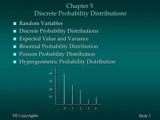
Some terminology • Random variable • A variable the values of which are determined by chance. • Examples of random variables • Number of heads in 10 tosses of a coin • Test score of students • Height • Income
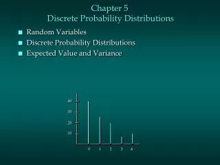
Probability distribution (function) • Shows the frequency (or chance) or occurrence of each value of the random variable.
Probability Distribution of Coin Toss - 1 • Slide 8 shows the empirical probability distribution. • Theoretical one can be computed • See animated demo Binomial Probability_demo.swf
Probability Distribution of Coin Toss - 2 Theoretical probabilities
How can we use the probability distribution - 1? • Provide information about “central tendency” (where the middle is, typically captured by Mean or Median), and variation (typically captured by standard deviation).
How can we use the probability distribution - 2? • Use the distribution as a point of reference • Example: • If we find that, 20% of the time, we obtain only 1 head in 10 coin tosses, when the theoretical probability is about 1%, we may conclude that the coin is biased (not 50-50 chance of tossing a head) • Theoretical distribution will be better than empirical distribution, because of fluctuation in the collection of data.
Random variables that are continuous • Collect a sample of height measurement of people. • Form an empirical probability distribution • Typically, the probability distribution will be a bell-shaped curve. • Compute mean and standard devation • Empirical distribution is obtained • Can we obtain theoretical distribution?
Normal distribution - 2 • A random variable, X, that has a normal distribution with mean and standard deviation can be transformed to a variable, Z, that has standard normal distribution where the mean is 0 and the standard deviation is 1. • z-score • Need only discuss properties of the standard normal distribution
Standard normal distribution - 1 5% in this region 2.5% in this region -1.64 1.96
Standard normal distribution - 2 • 2.5% outside 1.96 • So around 5% less than -1.96, or greater than 1.96. • So the general statement that Around 95% of the observations are within -2 and 2. • More generally, around 95% of the observations are within -2 and 2 (± 2 standard deviations).
Standard normal distribution - 3 • Around 95% of the observations lie within ± two standard deviations (strictly, ±1.96) 95% in this region
Standard normal distribution - 3 • Around 68% of the observations lie within ± one standard deviation 68% in this region
Computing normal probabilities in EXCEL • See animated demo NormalProbability_demo.swf
Exercise - 1 • For the data set distributed in Week 2, TIMSS2003AUS,sav, for the variable bsmmat01 (second last variable, maths estimated ability), compute the score range where the middle 95% of the scores lie: • Use the observed scores and compute the percentiles from the observations • Assume the population is normally distributed
Exercise - 2 • Dave scored 538. What percentage of students obtained scores higher than Dave? • Use the observed scores and compute the percentiles from the observations • Assume the population is normally distributed