Download
1 / 12
120 likes | 235 Views
Lecture 5 Moving from the AK model to the Solow model Gains from Specialization. Is the AK model too optimistic?

E N D
Lecture 5 Moving from the AK model to the Solow model Gains from Specialization
Is the AK model too optimistic? One of the optimistic assumptions of the AK model is that geometric growth continues forever on the basis of capital accumulation. With a production function Y = AK, the growth equation becomes: Y(t+1) = (1 + sA - d) Y (t) The growth rate, defined as g = [Y(t+1) – Y(t)]/Y(t) , then equals: g = sA - d The reason for this optimistic conclusion is the optimistic assumption regarding the benefits of capital accumulation. Every time the capital stock doubles, the output is assumed to double as well. The economy never becomes “saturated” with capital. The production function can be graphed as follows:
A less “optimistic” model Today we consider the important implications of a less “optimistic” view of capital accumulation. We now suppose that when the capital stock doubles, output less than doubles. A convenient mathematic form for such an assumption is the following: Y = A KB where B < 1 Notice that if B is equal to 1 then we are back in the “AK” Model. When B is less than 1 then we say that Y exhibits “diminishing marginal returns” in capital. This means that the gain from one extra unit of capital is less when there is a lot of capital than when there is not a lot of capital. The graph of this production function in the case that B = 0.25 is shown in the following figure.
Now, let’s study the growth process in this new case. As in the AK model we have a production function: Y = A K B We have the same expression relating investment to savings as before: I = s Y And we have the same law that governs the accumulation of capital: K(t+1) = K(t) + s Y - d K(t) With our new production function this expression is now written: K(t+1) = K(t) + s A K(t) B - d K(t)
Assuming that the initial capital stock in year 2001 is K(2001)=1, we now have everything we need to graph the capital stock as a function of time. It looks like this.
…and once we know what the capital stock is at every point in time we can use our production function to work out what the income level is at every point in time. It looks like this:
Notice that growth is no longer self-sustaining! As K gets large, the saving from additional K (equal to s times the increase in output) just balances the additional depreciation on capital, so that there is no NET gain in the capital stock. In mathematical terms we have: K(t+1) - K(t) = s A K B - d K If there is no increase (or decrease) in the capital stock then the left hand side of this expression is equal to 0. But then the right habd side equals 0. In other words: s A K B = d K That is, the amount of saving is exactly equal to the amount of depreciation.The value of K(t+1) – K(t) is graphed below as a function of K.
Increased Income Due to Specialization Average output per capita rises when the division of labor is increased, because of the gains to specialization. To see how this works we can again use a “mathematical model” Suppose that there are just two individuals, person 1 and person 2. They each work for 40 hours each week. Hence we may write their labor as L1 = 40 L2 = 40 Each individual consumes two goods: food and clothing, and they like to consume these in equal amounts. To produce food requires 10 hours to set up, and then 1 hour for each unit of food that is produced. If the worker spends half his work week (20 hours) making food, he would set up for 10, and then produce for 10, making 10 units of food.
To produce clothing also requires 10 hours to set up, and then 1 hour for each unit of clothing is produced. If the worker spends half his work week (20 hours) making clothing, he would set up for 10, and then produce for 10 hours, making 10 units of clothing. Thus, a worker working in isolation, and dividing his time between the two activities, ends up with 10 units of food, and 10 units of clothing. Now, suppose that one worker specializes in food, and one worker specializes in clothing. They then trade half of their output to the other person, so that they end up with equal amounts of food and clothing. The first worker producing food requires 10 hours to set up and then produces 30 units of food. The second worker producing clothing requires 10 hours to set up and then produces 30 units of clothing. They trade half of their output to the other, each ending up with 15 units of food and 15 units of clothing. Instead of a collective 40 hours of set up time, as when they work in isolation, the collective set-up time is reduced to 20 hours, and the extra twenty hours of work time produces 5 units more of food and clothing for each worker.