Download
1 / 50
530 likes | 662 Views
Temporal resolution. The ability to follow rapid changes in a sound over time. The bottom line. People manage to maintain good temporal resolution without compromising sensitivity by using intelligent processing.

E N D
Temporal resolution The ability to follow rapid changes in a sound over time
The bottom line People manage to maintain good temporal resolution without compromising sensitivity by using intelligent processing.
Temporal resolution: How good is a listener at following rapid changes in a sound? • Auditory nerve fibers do not fire at the instant at which sounds begin or end. • Auditory nerve fibers do not fire on every cycle of sound. • Adaptation occurs to longer duration sounds. • Spontaneous activity occurs when no sound is present
Following rapid changes in sound The auditory nerve response does not follow changes with perfect precision
AVERAGE Firing rate Firing rate Time Time Averaging over time is one way the auditory system could “smooth out” the bumpy response of auditory nerve fibers
AVERAGE Firing rate Firing rate Time Time The time over which you average makes a difference Long time averaging AVERAGE Firing rate Short time averaging Firing rate Time Time
The temporal window 1 2 5 3 4 4 5 3 2 1 pressure Averaged Firing rate (s/s) Time Time (ms)
The temporal window 2 1 pressure 1 2 Firing rate (s/s) Time Time (ms)
Hydraulic analogy: How long before the next bucket leaves for the brain? Inner HC Auditory nerve fiber To the Brain
Hydraulic analogy: How long before the next bucket leaves for the brain? Inner HC Auditory nerve fiber To the Brain
People can “add up” sound energy for • 5 ms • 50 ms • 200 ms • 1500 ms 11
Temporal resolution: How short are the “samples” of sound? Hypothesis # 1: We integrate over 200-300 ms. From Gelfand (1997)
Sensitivity-resolution tradeoff If you extend the integration time to improve sensitivity, you lose resolution.
So how well should I be able to discriminate a change in the duration of a sound? v. Level (dB) Level (dB) 160 200 Time (ms) Time (ms) 40 ms difference ~ 1 dB--like the jnd
How to measure temporal resolution • Duration discrimination • Gap detection • Amplitude modulation detection
Amplitude (dPa) Level (dB) - Forever Forever Frequency (Hz) Time (ms) Problem in measuring temporal resolution: “Spectral splatter” Amplitude (dPa) Level (dB) Frequency (Hz) 5 0 Time (ms)
Level (dB) Level (dB) Time (ms) Time (ms) Duration discrimination Interval 2 Interval 1 Which gap was longer?
Duration discrimination • Weber’s Law? NO • Duration discrimination can be very acute - much better than 50-75 ms. From Yost (1994)
Level (dB) Level (dB) Time (ms) Time (ms) Gap detection Interval 2 Interval 1 Which one had a gap?
Masking spectral splatter Gap detection From Moore (1997)
Firing rate Firing rate Level (dB) Time (ms) Time (ms) Time (ms) Is it temporal resolution or intensity resolution? Good intensity resolution Nice long gap Bad intensity resolution
Amplitude modulation detection By how much do I have to modulate the amplitude of the sound for the listener to tell that it is amplitude modulated, at different rates of modulation?
Modulation depth 25% 100% 50
Time Not AM AM Respond: 1 or 2? Respond: 1 or 2? Respond: 1 or 2? Warning Warning Warning Interval 2 Interval 2 Interval 2 Interval1 Interval1 Interval1 1 2 2 Trial1 Trial3 Trial2 2AFC AM Detection Feedback Which one was AM? Vary depth of AM to find a threshold
AM detection as a function of modulation rate The temporal modulation transfer function (TMTF) From Viemeister (1979)
What sort of filter has a response that looks like this? • low-pass • high-pass • bandpass • band reject Level (dB) Frequency (Hz) 28
The TMTF is like a low-pass filter. That means that we can’t hear • slow amplitude modulations • high frequencies • low frequencies • fast amplitude modulations 29
About 3 dB About 3 dB About 3 dB TMTF at different carrier frequencies From Viemeister (1979)
Conclusions from TMTF • People are very good at AM detection up to 50-60 Hz modulation rate (and intensity resolution effects are controlled) • 50-60 Hz = 17-20 ms/cycle of modulation • 17-20 ms < 40 ms • Somehow the auditory system is getting around the sensitivity-resolution tradeoff
The auditory system can follow amplitude modulation well up to about • 50-60 Hz • 120 Hz • 4 Hz • 2000 Hz 32
So how can we detect such short changes in a sound and still be able to integrate sound energy over 200-300 ms?
Two theories of temporal resolution-temporal integration discrepancy • Multiple integrators • Multiple looks
Multiple integrators Inner HC Buckets leave every 200 ms AN fiber 1 Buckets leave every 100 ms AN fiber 2 Buckets leave every 50 ms AN fiber 3 To the Brain Etc. Etc.
Inner HC For detecting sounds To the Brain Multiple integrators Buckets leave every 200 ms AN fiber 1 Buckets leave every 100 ms AN fiber 2 Buckets leave every 50 ms AN fiber 3 Etc. Etc.
For detecting gaps Multiple integrators Inner HC Buckets leave every 200 ms AN fiber 1 Buckets leave every 100 ms AN fiber 2 Buckets leave every 50 ms AN fiber 3 To the Brain Etc. Etc.
AN fibers don’t have different integration times But of course the integrators could be somewhere else in the brain.
Buckets leave every 50 ms Buckets leave every 50 ms Buckets leave every 50 ms Multiple looks In the brain... Inner HC AN fiber 1 AN fiber 2 AN fiber 3 Memory: Hold on to those buckets for 200 ms and check them out To the Brain Etc. Etc.
Multiple looks theory says • we have good temporal resolution because we use memory to integrate sound “energy” • we have good temporal resolution because we have some neurons that have good temporal resolution and some neurons that don’t.
Multiple integrators theory says • we have good temporal resolution because we use memory to integrate sound “energy” • we have good temporal resolution because we have some neurons that have good temporal resolution and some neurons that don’t.
A test of the multiple looks theory: Viemeister & Wakefield (1991) Set up a situation in which the two theories predict different outcomes...
Viemeister & Wakefield (1991) It would be useful to integrate the 2 tone pips to improve detection, and both theories say you could do that.
Viemeister & Wakefield (1991) But if you put noise on between the tone pips, you can’t integrate them without integrating in the noise. If you’re taking short looks, you can use the looks with the tone pips, but ignore the looks in between.
Viemeister & Wakefield (1991) Multiple integrator “performance” will get worse if the noise goes up more, and better if the noise goes down some, but multiple looks are not affected by what happens between the tone pips.
The results of Viemeister & Wakefield are most consistent with • multiple looks theory • multiple integrators theory 47
Conclusions • People can detect very short duration changes in sound, such as 2-3 ms long interruptions. • People can integrate sound energy over 200-300 ms to improve sound detection. • The auditory system gets around the sensitivity-resolution tradeoff by using short-term integration and intelligent central processing.
Text sources • Gelfand, S.A. (1998) Hearing: An introduction to psychological and physiological acoustics. New York: Marcel Dekker. • Moore, B.C.J. (1997) An introduction to the psychology of hearing. (4th Edition) San Diego: Academic Press. • Viemeister, N.F. (1979). Temporal modulation transfer functions based upon modulation thresholds. J. Acoust. Soc. Am., 66, 1564-1380. • Viemeister, N.F. & Wakefield, G. (1991) Temporal integration and multiple looks. J. Acoust. Soc. Am., 90, 858-865. • Yost, W.A. (1994) Fundamentals of hearing: an introduction. San Diego: Academic Press.
Text sources • Gelfand, S.A. (1998) Hearing: An introduction to psychological and physiological acoustics. New York: Marcel Dekker. • Moore, B.C.J. (1997) An introduction to the psychology of hearing. (4th Edition) San Diego: Academic Press. • Viemeister, N.F. (1979). Temporal modulation transfer functions based upon modulation thresholds. J. Acoust. Soc. Am., 66, 1564-1380. • Viemeister, N.F. & Wakefield, G. (1991) Temporal integration and multiple looks. J. Acoust. Soc. Am., 90, 858-865. • Yost, W.A. (1994) Fundamentals of hearing: an introduction. San Diego: Academic Press.