Download
1 / 18
180 likes | 184 Views
Combating Dissipation. Numerical Dissipation. There are several sources of numerical dissipation in these simulation methods Error in advection step Pressure projection (time splitting) Not addressed yet in graphics! Level set redistancing Focus on the first. Dissipation Example (1).

E N D
Numerical Dissipation • There are several sources of numerical dissipation in these simulation methods • Error in advection step • Pressure projection (time splitting) • Not addressed yet in graphics! • Level set redistancing • Focus on the first
Dissipation Example (1) • Start with a function nicely sampled on a grid:
Dissipation Example (2) • The function moves to the left(perfect advection) and is resampled
Dissipation Example (3) • And now we interpolate from new sample values, and ruin it all!
The Symptoms • For velocity: • Too viscous or sticky (molasses), or at an implausible length scale (scale model) • Turbulent detail quickly blurred away • For smoke concentration: • Smoke diffuses into thin air too fast,nice sharp profiles or thin features vanish • For level sets: • Water evaporates into thin air, bubbles disappear
High Order/Resolution Schemes • That said, we can do a lot better thanfirst-order semi-Lagrangian • High order methods: use more data points to get more accurate interpolation • Cancel out more terms in Taylor series • Problem: inevitably can give undershoot/overshoot (too aggressive) • Stability for nonlinear problems? • High resolution methods: high order except near sharp regions
Sharpening semi-Lagrangian • Can also do better with semi-Lagrangian approach • Sharper interpolation- e.g. limited Catmull-Rom [Fedkiw et al ‘02] • Estimating error and subtracting it • BFECC [e.g. Kim et al ‘05] • Using derivative information • CIP [e.g. Yabe et al. ‘01]
Example • Exact (particles) vs. 1st order vs. BFECC
Aside: resampling • Closely related to the sampling theorem:frequencies above a certain limit cannot be reliably recovered on a grid • Sharp features have infinitely high frequency! • Schemes which use an Eulerian grid as fundamental structure are inherently limited(forced to use higher resolution than is strictly necessary)
Particle-in-Cell Methods • Back to Harlow, 1950’s, compressible flow • Abbreviated “PIC” • Idea: • Particles handle advection trivially • Grids handle interactions efficiently • Put the two together:- transfer quantities to grid- solve on grid (interaction forces)- transfer back to particles- move particles (advection)
PIC • Start with particles • Transfer to grid • Resolve forces on grid • Gravity, boundaries, pressure, etc. • Transfer velocity back to particles • Advect: move particles • Start with particles • Transfer to grid • Resolve forces on grid • Gravity, boundaries, pressure, etc. • Transfer velocity back to particles • Advect: move particles
PIC • Start with particles • Transfer to grid • Resolve forces on grid • Gravity, boundaries, pressure, etc. • Transfer velocity back to particles • Advect: move particles • Start with particles • Transfer to grid • Resolve forces on grid • Gravity, boundaries, pressure, etc. • Transfer velocity back to particles • Advect: move particles
PIC • Start with particles • Transfer to grid • Resolve forces on grid • Gravity, boundaries, pressure, etc. • Transfer velocity back to particles • Advect: move particles
PIC • Start with particles • Transfer to grid • Resolve forces on grid • Gravity, boundaries, pressure, etc. • Transfer velocity back to particles • Advect: move particles
PIC • Start with particles • Transfer to grid • Resolve forces on grid • Gravity, boundaries, pressure, etc. • Transfer velocity back to particles • Advect: move particles
FLuid-Implicit-Particle (FLIP) • Problem with PIC: we resample (average) twice • Even more numerical dissipation than pure Eulerian methods! • FLuid-Implicit-Particle (FLIP) [Brackbill & Ruppel ‘86]: • Transfer back the change of a quantity from grid to particles, not the quantity itself • Each delta only averaged once: no accumulating dissipation! • Nearly eliminated numerical dissipation from compressible flow simulation… • Incompressible FLIP [Zhu&Bridson’05]
Where’s the Catch? • Accuracy: • When we average from particles to grid, simple weighted averages is only first order • Not good enough for level sets • Noise: • Typically use 8 particles per grid cell for decent sampling • Thus more degrees of freedom in particles then grid • The grid simulation can’t see/respond to small-scale particle variations – can potentially grow in time • Regularize: e.g. 95% FLIP, 5% PICCan actually determine ratio which matches a particular physical viscosity!