Download
1 / 35
350 likes | 361 Views
Program Analysis. Mooly Sagiv http://www.math.tau.ac.il/~sagiv/courses/pa.html Tel Aviv University 640-6706 Sunday 18-21 Scrieber 8 Monday 10-12 Schrieber 317 Textbook: Dataflow Analysis Chapter 2 & Appendix A Monotone Frameworks and Precision May 19, 10am Exam?. Outline.

E N D
Program Analysis Mooly Sagiv http://www.math.tau.ac.il/~sagiv/courses/pa.html Tel Aviv University 640-6706 Sunday 18-21 Scrieber 8 Monday 10-12 Schrieber 317 Textbook: Dataflow Analysis Chapter 2 & Appendix A Monotone Frameworks and Precision May 19, 10am Exam?
Outline • Monotone Dataflow Frameworks • Precision of Data Flow Analysis • Beyond Monotone Frameworks
Complete Lattices • The Poset (L, ) such that every subset SLS and S are both defined is called complete lattice • Denoted by (L, ) = (L, , , , ,) • is the minimum value • = = L • is the maximum value • = L =
Monotone Frameworks • Generalizes Kill/Gen Problems • A complete lattice (L, , , , ,) describes the “potential pieces of information” • The initial value at entry is specified by L • The effect of every basic block at l is described by a monotone function fl :L L (transfer function) • Solve the following system of equations (forward)
Monotone Backward Frameworks • A complete lattice (L, , , , ,) describes the “potential pieces of information” • The initial value at exit is specified by L • The effect of every basic block at l is described by a monotone function fl :L L (transfer function) • Solve the following system of equations
Instances of Monotone Frameworks • Kill/Gen Problems • = or = • fl(entry(l)) = (entry(l) - kill(l)) gen(l) • Forward • May be uninitialized (garbage) variables • Constant propagation • Sign-analysis • Parity analysis • Points-to analysis • Backward • Truly-live variables
May-be-garbage variables • A variable may-be-garbage at a labell if there may be a path to l in which it is either uninitialized or set using an uninitialized variable[x := 5]1 ;if [z > 2]2 then [y := 17]3 ; else [skip]4 ;[t := y + x]5 ;
May-be-garbage variables(cont) • L = (P(Var*), , , , , Var*) • Initial value =Var* • Transfer functions
The Factorial Program [y := x]1;[z := 1]2; while [y>1]3 do ( [z:= z * y]4; [y := y - 1]5; ) [y := 0]6;
Over Conservative Solution if [y >1]1 then [z := 1]2; … if [y >1]3 then [y := z]4;
ConstantPropagation • Determine variables with constant values • Information Lattice • Extended integer lattice (L1, 1, 1, 1, 1, 1) • L1 = Z {1, 1} • 1 1 z1 1 • Define L = (S L1, ) where S=Var* • Initial value ? • Transfer functions Acp: AExp (LL1)
The Factorial Program [y := x]1;[z := 1]2; while [y>1]3 do ( [z:= z * y]4; [y := y - 1]5; ) [y := 0]6;
[y := 5]1;[x := 8]2;while [x>1]3 do ( [x:= y+3]4; [x := (y * y) -17]5; )
ParityAnalysis • Determine parity of a single variable x • Information Lattice • ({E, O, , } , , , , , ) • z • ‘E’ denotes the fact that x is even • ‘O’ denotes the fact that is x is odd • Initial value = • Transfer functions • Expressions • Statements • Conditions
Example Program • while [x !=1]1 do if [ (x %2) = 0]2 then [x := x / 2;]3 else [x := x * 3 + 1;]4
Example Program • while/*[x ]*/ [x !=1]1 /*[x ]*/ do if /*[x ]*/ [ (x %2) = 0]2 then/*[x E]*/ [x := x / 2;]3 /*[x ]*/ else /*[x O]*/ [x := x * 3 + 1;]4 /*[x E]*/
The PWhile Programming Language Abstract Syntax a := x | *x | &x | n | a1 opa a2 b := true | false | not b | b1 opb b2 | a1 opr a2 S := [x := a]l | [*x := a]l | [skip] l | S1 ; S2|if [b]lthen S1else S2 | while [b]l do S
Points-ToAnalysis • Determine if a pointer variable p may point to q • L = (P(Var* Var*), , , , , Var* Var*) • (x, y) l --- x may hold the address of y • The initial value = • Transfer functions
Usage of Points-To-Information • “Adapt” other optimizations • Constant propagationx = 5;*p = 7 ;… x … • Pointer aliases • Variables p and q are may-aliases at l if the points-to set at l contains entries (p, x) and (q, x) • Side effect analysis *p = *q + * * t
[t := &a]1; [y := &b]2; [z := &c]3; if [x> 0]4; then [p:= &y]5; else [p:= &z]6; [*p := t]7;
/* */ [t := &a]1; /* {(t, a)}*/ /* {(t, a)}*/ [y := &b]2; /* {(t, a), (y, b) }*/ /* {(t, a), (y, b)}*/ [z := &c]3;/* {(t, a), (y, b), (z, c) }*/ if [x> 0]4; then [p:= &y]5;/* {(t, a), (y, b), (z, c), (p, y)}*/ else [p:= &z]6; /* {(t, a), (y, b), (z, c), (p, z)}*//* {(t, a), (y, b), (z, c), (p, y), (p, z)}*/ [*p := t]7; /* {(t, a), (y, b), (y, c), (p, y), (p, z), (y, a), (z, a)}*/
Chaotic Iterationsfor forward problems for l Lab*do DFentry(l) := DFexit(l) := DFentry(init(S*)) := WL= Lab* while WL != do Select and remove an arbitrary l WL if (temp != DFexit(l)) DFexit(l) := temp for l' such that (l,l') flow(S*) do DFentry(l') := DFentry(l') DFexit(l) WL := WL {l’}
Chaotic Iterationsfor backward problems for l Lab*do DFentry(l) := DFexit(l) := for l final(S*)) do DFexit(l) := WL= Lab* while WL != do Select and remove an arbitrary l WL if (temp != DFentry(l)) DFentry(l) := temp for l' such that (l’, l) flow(S*) do DFexit(l') := DFexit(l') DFentry(l) WL := WL {l’}
Complexity of Chaotic Iterations • Parameters: • |Lab| labels • k is the maximum outdegree of flow(S*) • A lattice of height h • c is the maximum cost of • applying fl • • L comparisons • ComplexityO(|Lab| h * c * k)
Soundness of Chaotic Iterations • define a monotone abstraction : Collecting-States L • Show that for every l: • ({[b]l(s) | s CS }) fl ((CS)) • Conclude that the DF solution of Chaotic iterations satisfies for every l: • (CS entry(l)) DFentry(l) • (CS exit(l)) DFexit(l) • But it may be that Chaotic iterations yield DFentry(l) = and yet (CS entry(l))= • How to measure precision?
Precision of Chaotic Iterations • Optimal • (CS entry(l)) = DFentry(l) • (CS exit(l)) = DFexit(l) • Join-over-all-paths - No loss of information w.r.t. straight line code • Relatively optimal (induced) w.r.t. the abstraction • Compare at run-time • Good enough for the used optimization
The Join-Over-All-Paths (JOP) • Let paths(init(S*), l) denote the potentially infinite set of paths from init(S*) to l (written as sequences of labels) • For a sequence of labels [l1, l2, …, ln] definef [l1, l2, …, ln]: L L by composing the effects of basic blocks • f[l](s)=s • f[l, p](s) = f[p](fl(s)) • JOPl = {f[l1, l2, …, l]() [l1, l2, …, l] paths(init(S*), l)}
JOP vs. Least Solution • The DF solution obtained by Chaotic iteration satisfies for every l: • JOPl DFentry(l) • If every fl is additive (distributive) for all the labels l • JOPl= DFentry(l)
Additive (Distributive)Monotone Problems • Kill/Gen Problems • May-be uninitialized • Truly-live variables • Constant Propagation when every expression in the right hand side contains at most one variable • Points-to analysis with one level pointers
Non DistributiveMonotone Problems • Points-to-analysis • Constant Propagation on arbitrary expressions • Parity Propagation on arbitrary expressions
Converting into Distributive Frameworks • Consider • a finite lattice (L, , , , ,) • An initial value at entry L • The effect of every basic block at l is described by a monotone function fl :L L (transfer function) • Define a distributive function on (P(L), , , , , L) by • Solve the following system of equations over P(L)
The Constant Propagation • It is undecidable to find the JOP in the constant propagation problem • A Sketch of a proof while (...) ( if (...) x_1 = x_1 + 1; if (...) x_2 = x_2 + 1; ... if (...) x_n = x_n + 1; } y = truncate (1/ (1 + p2(x_1, x_2, ..., x_n))/* Is y=0 here? */
Static Analysis problems beyond Monotone Frameworks • Infinite heights • integer intervals • Linear relationships between variables • Bi-directional problems • Partial-redundant expressions • Automatic inference of variable types in imperative (weakly typed) programs x := b[z] a [b[y]] := x • Procedures
Historical Perspective • 1973 Kildall defined the basic framework but required distributive frameworks • 1976 Kam and Ulmann defined Monotone Framework • 1980 Tarjan suggested an almost linear time algorithm for reducible flow graph • 1980 Rosen suggested a linear time algorithm for high level language
Conclusions • Many dataflow problems can be solved via the Chaotic Iteration Algorithm • Provide a tool to understand precision