Download

1 / 20
200 likes | 205 Views
ENVE3503 Environmental Engineering. Groundwater Supply. Dr. Martin T. Auer Michigan Tech Department of Civil & Environmental Engineering. Drinking Water Sources.

E N D
ENVE3503 Environmental Engineering Groundwater Supply Dr. Martin T. Auer Michigan Tech Department of Civil & Environmental Engineering
Drinking Water Sources Approximately two-thirds of the population of the U.S. receives its supply from surface waters. However, the number of communities supplied by groundwater is four times that supplied by surface water. This is because large cities are typically supplied by surface waters and smaller communities use groundwater.
An Aquifer water table water table well vadose zone capillary fringe unconfined aquifer water table impermeable layer
Unconfined Aquifer water table unconfined aquifer re-charge water table well unconfined aquifer water table – piezometric surface where water pressure equals atmospheric pressure Unconfined Aquifer manometer
Confined Aquifer confined aquifer re-charge piezometric surface piezometric surface confined aquifer = f (K) confining layer aquiclude Confined Aquifer
Confined Aquifer water table unconfined aquifer re-charge water table well • Unconfined aquifer • zone of aeration • zone of saturation • vadose zone • capillary fringe • water table • water table well • re-charge zone • Confined aquifer • piezometric surface • confining layer • artesian well • re-charge zone unconfined aquifer Confined Aquifer confined aquifer re-charge piezometric surface = f (K) confined aquifer confining layer
Cone of Depression cone of depression aquaclude = impermeable layer
Effect of Pumping Rate drawdown radius of influence
Porosity and Packing Small soil particles pack together more closely than large particles, leaving many small pores. Large soil particles pack together less closely, leaving fewer, but larger, pores. A given volume of spherical solids will have the same porosity, regardless of the size of the particles. The significance of porosity lies in role of surface tension (higher for small pores) in retaining water and frictional losses in transmitting water. Most soils are a mixture of particle sizes. Poorly sorted soils (greater range of particle sizes) will have a lower porosity, because the smaller particles fill in the "gaps“.
Porosity of Specific Soils Clays are small soil particles and thus one would expect tight packing. However, the net negative charge of clay particles separates them, resulting in a higher porosity than for a sphere of equivalent volume. Silts are intermediate in size between clays and sands and are irregular in shape. This irregularity leads to poorer packing than for spherical particles of similar volume and thus a higher than expected porosity. Sands are large particles, more regular in shape than silts and thus having a porosity similar to that expected for spherical particles.
Porosity Values The net effect of the physicochemical properties of clay, silt and sand particles is that the porosity and thus water content tends to decrease as particle size increases. soil particles pores
Specific Yield This is the amount of water, expressed as a %, that will freely drain from an aquifer
Specific Yield Having a lot of water does not mean that an aquifer will yield water. Surface tension effects, most significant in soils with small pores, tend to retain water reducing the specific yield. A better expression of the water available for development in an aquifer is the ratio of specific yield to porosity.
Hydraulic Gradient Darcy’s Law hydraulic conductivity
Hydraulic Conductivity (a.k.a. coefficient of permeability) K = m3·m-2·d-1 = m·d-1
M1 M2 E S2 S1 H h2 h1 h = H - s r1 r2 Determining Hydraulic Conductivity An extraction well (E) is pumped at a constant rate (Q) and the drawdown (S) is observed in two monitoring wells (M) located at a distance (r) from the extraction well. Determination of Hydraulic Conductivity Hydraulic conductivity (m3∙m-2∙d-1) is then calculated by solving Darcy’s Law to yield:
h = H - s E S2 h1 H h2 S1 r1 r2 Estimating Well Production At maximum drawdown, conditions at r1 (the well radius) are s1 = H and h1 = 0 and conditions at r2 (the edge of the cone of depression) are s2 = 0 and h2 = H. And the maximum pumping rate (m3∙d-1) is calculated using the equation below: