Reconstruction on trees and Phylogeny 2

1. Reconstruction on trees and Phylogeny 2 Elchanan Mossel, U.C. Berkeley mossel@stat.berkeley.edu, http://www.cs.berkeley.edu/~mossel/ Supported by Microsoft Research and the Miller Institute

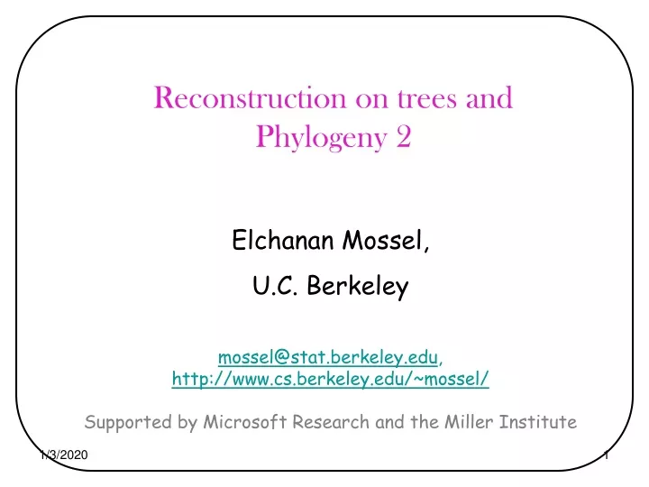
2. Reconstruction on Ising-CFN model • We study the reconstruction problem for the Ising-CFN model on regular trees. + + + + - + + - - + - + + +

3. Markov models on trees Finite set A of information values. Tree T=(V,E) rooted at r. Vertex v 2 V, has information σv2 A. Edge e=(v, u), where v is the parent of u, has a mutation matrix Me of size |A| £ |A|: Mi,j (v,u) = P[u = j | v = i] For each character , we are given T = (v)v 2T, where T is the boundary of the tree. We will focus on the Ising-CFN model:

4. Statistical physics Statistical physics is a sub-field of mathematical physics where we study complex systems with simple microscopic interactions. The Ising model on a graphis a probability measure (“Gibbs distribution”) on the space of configurations σ from vertices to {-1,1} such that P[σ] ~ exp(Σ(v, w) ε E σ(v)σ(w)/T). Traditionally studied on cubes in Zd. The Ising model on 200 x 200 grid

5. Statistical physics on trees The Ising model on the binary tree can be defined: Set σr, the root spin, to be +/- with probability ½. For all pairs of (parent, child) = (v, w), set σw = σv, with probability , otherwise σw = +/- with probability ½. This is exactly the CFN model. • Studied in statistical physics [Spitzer 75, Higuchi 77, Bleher-Ruiz-Zagrebnov 95, Evans-Kenyon-Peres-Schulman 2000, Ioffe 99, M 98, Haggstrom-M 2000, Kenyon-M-Peres 2001, Martinelli-Sinclair Weitz 2003, Martine 2003] + + + + - + + - - + - + + +

6. Reconstruction solvability Let T be an infinite rooted tree and Tn denote the first n levels of T. We say that the reconstruction problem is solvable if one of the following equivalent conditions hold: 9 s.t. (8 non-degenerate ) limn !1 I(X0,Xn) > 0, where I(X0,Xn) = H(X0) + H(Xn) – H(X0,Xn); H is the entropy operator, H(X) = -x P[X = x] log2 P[X = x]. 9 i,j s.t. limn !1 | Pni - Pnj | > 0, where Pnj denotes the distribution of Xn conditional on X0 = j. If X0 has the uniform distribution then, liminfn !1n > 1/m, where n is the probability of correct reconstruction of X0 given Xn. 9 (8 non-degenerate ) liminfn !1 Var[E[X0|Xn]] > 0.

7. The Ising model on the 3-regular tree mutual information: H(σ∂) + H(σr)) - H(σr,σ∂)

8. Reconstruction for the CFN model • Thm: The reconstruction problem for the Ising model on the (b+1)-regular tree is solvable if and only ifb 2 > 1. • “Easy direction” [Higuchi 77]: prove that a certain reconstruction algorithm works when b 2 > 1. • Higuchi argument extends to general chains and general trees. • Will also show an argument from [M98] useful for phylogeny. • “Hard direction” [¸ 95]: Non-reconstruction? • 6 different proofs! • All involve a magic. • None extends to other markov models. • Will follow a coupling proof [Martinelli-Siclair-Weitz]

9. Non-reconstruction - Coupling down • Copying rule. For i =+,-: • P[i ! i] = . • P[i ! Uniform] = 1 – . • Continuing down the tree, non-coupled elements form a branching process with parameter . + / - + / - = = + / - = = = = = = = = = = • If b · 1, branching process dies)coupling. • More generally, at level n, the expected number of uncoupled sites is bnn. • (Doesn’t work all the way to b 2· 1).

10. Non-reconstruction - Coupling up • We try to couple two configurations which differ at level n so that they agree at the root. • First consider the case where they differ at exactly one site. = = + / - u v = = = = + / - = = = • Lemma [Mossel-Kenyon-Peres]: Among all boundary conditions,E [u = 1 | v = 1] – E[u = -1 | v = 1] is maximized for the free boundary. • )P[not coupling at u] ·. • )P[not coupling at the root] ·n.

11. Coupling up – path coupling • We got that if  and  are two boundary conditions which differ in one position at level n, then • |E[()] – E[()] · 2 n, where  is the root. • )if  and  are two boundary conditions which differ at k sites, then • |E[()] – E[()] · 2 k n. • Pf: If  and  differ at k sites, then we can find a sequence  = (0),(1),…,(k) = , such that i and i+1 differ in exactly one site. • |E[()] – E[()] · • i=1k |E(i)[()] – E(i-1)[()]| · 2 k n.

12. Non reconstruction for b 2 < 1 • Fix  such that b 2 < 1. • We will show that E+[E[() | +]] – E-[E[() | -] ! 0, • where + =boundary conditions conditioned on () = +. • Let (+,-) be given by the “down coupling”. • Let K(+,-) = number of disagreements between +,-. • E+[E[() | +]] – E- E[() | -]] • = E_{+,-}[E[() | +] - E[() | -]] • ·E+,-[2 K(+,-) n] = 2 n E+,-[K(+,-)] (“up coupling”). • = 2 n£ bnn (“down coupling”) • = 2 (b 2)n! 0exp. fast in n.

13. Where we stopped … • Thm: The reconstruction problem for the Ising model on the (b+1)-regular tree is solvable if and only ifb 2 > 1. • We showed that if b 2 < 1, it is impossible to reconstruct (“hard” direction). • We now show that if b 2 > 1, we can reconstruct.

14. Reconstruction via majority • Fix  such that b 2 > 1. • Let X =Xn = #(+) - #(-) at level n. • We claim that Xn is a good estimator of (). • E+[Xn] = bnn ; E-[Xn] = -bnn. • We show that E+/-[Xn2] · c(E+/-[Xn])2 = c b2n2n. • Let f = fn (g = gn) be the density of the + (-) measure with respect to some reference measure . • 2 bnn = E+[X] – E-[X] = s X (f – g) d  = • = s X (f1/2 – g1/2) (f1/2 + g1/2) d  • ·(s X2 (f1/2 + g1/2)2 d)1/2£ (s (f1/2 – g1/2)2 d )1/2 • ·(4 s X2 f d+ 4 s X2 g d)1/2£ (s |f – g| d)1/2 • ·(8 c b2n2n)1/2 (DTV(+,-))1/2.

15. Bounds on the second moment • Write Xn = v(v), where the sum is over all v in level n. • E+[Xn2] = v,w E+[(v) (w)]. • For each edge with prob.  the two end points are the same and with prob. 1- the two points are independent. • If there is a red edge on the path between v and w, then E+[(v) (w)] = 0. v w v w • Otherwise, (v) = (w). • E+[(v) (w)] = d(v,w). • E+[Xn2] = bn(1 + i=1n (bi – bi-1)2i) • = bn(1 + (b-1) 2 i=0n-1 bi 2i). • = O(b2n 2n) iff b 2 > 1. v 1 2 4

16. Remarks on the second moment • Kamea/ Higuchi argument is very robust. • Works for general trees when br(T) 2 > 1. • Works for general markov chains, where  = 2nd eigenvalue of M (M-Peres 2002). • Kesten-Stigum (1966!) proved that for all markov chains • if b 2 > 1, then the limiting law of the count depends on the root. • If b 2 < 1, then the limiting law is normal for all root values. • M-Peres (2002)count reconstruction is impossible if b 2 < 1.

17. Recursive reconstruction for Ising models  • An alternative proof for reconstruction for b 2 > 1[M98] • Advantage: Works also when we have lower bound on . Majority doesn’t. • Blue edges have 1 , black2,1 < 2 ~ 1. • Maj(σ∂) ~ Maj of black tree. • Maj of black tree ~σv . • σv andσhave exp. small correlation. • Phylogeny: reconstruction given bounds. v • Instead we will use recursive-majority.