Iterative Improvement

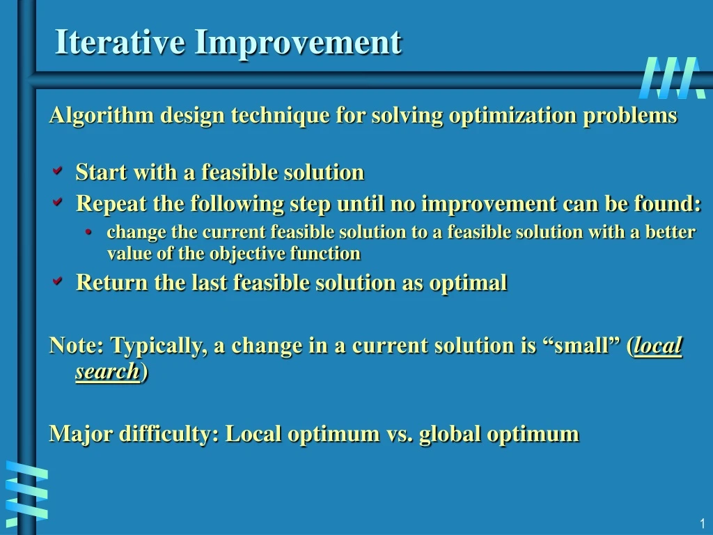
1. Iterative Improvement Algorithm design technique for solving optimization problems • Start with a feasible solution • Repeat the following step until no improvement can be found: • change the current feasible solution to a feasible solution with a better value of the objective function • Return the last feasible solution as optimal Note: Typically, a change in a current solution is “small” (local search) Major difficulty: Local optimum vs. global optimum

2. Important Examples • simplex method • Ford-Fulkerson algorithm for maximum flow problem • maximum matching of graph vertices • Gale-Shapley algorithm for the stable marriage problem • local search heuristics

3. Linear Programming Linear programming (LP) problem is to optimize a linear function of several variables subject to linear constraints: maximize (or minimize) c1 x1 + ...+ cnxn subject to ai 1x1+ ...+ ainxn ≤ (or ≥ or =) bi , i = 1,...,m x1≥ 0, ... , xn ≥ 0 The function z = c1 x1 + ...+ cnxn is called the objective function; constraints x1≥ 0, ... , xn ≥ 0 are called nonnegativity constraints

4. Example maximize 3x + 5y subject to x + y ≤ 4 x + 3y ≤ 6 x ≥ 0, y ≥ 0 Feasible region is the set of points defined by the constraints

5. Geometric solution maximize 3x + 5y subject to x + y ≤ 4 x + 3y ≤ 6 x ≥ 0, y ≥ 0 Optimal solution: x = 3, y = 1 Extreme Point Theorem Any LP problem with a nonempty bounded feasible region has an optimal solution; moreover, an optimal solution can always be found at an extreme point of the problem's feasible region.

6. 3 possible outcomes in solving an LP problem • has a finite optimal solution, which may no be unique • unbounded: the objective function of maximization (minimization) LP problem is unbounded from above (below) on its feasible region • infeasible: there are no points satisfying all the constraints, i.e. the constraints are contradictory

7. The Simplex Method • The classic method for solving LP problems; one of the most important algorithms ever invented • Invented by George Dantzig in 1947 • Based on the iterative improvement idea: Generates a sequence of adjacent points of the problem’s feasible region with improving values of the objective function until no further improvement is possible

8. Standard form of LP problem • must be a maximization problem • all constraints (except the nonnegativity constraints) must be in the form of linear equations • all the variables must be required to be nonnegative Thus, the general linear programming problem in standard form with m constraints and n unknowns (n ≥ m) is maximize c1 x1 + ...+ cnxn subject to ai 1x1+ ...+ ainxn = bi , i = 1,...,m, x1≥ 0, ... , xn ≥ 0 Every LP problem can be represented in such form

9. Example maximize 3x + 5y maximize 3x + 5y + 0u + 0v subject to x + y ≤ 4 subject to x + y + u = 4 x + 3y ≤ 6 x + 3y + v = 6 x≥0, y≥0 x≥0, y≥0, u≥0, v≥0 Variables u and v, transforming inequality constraints into equality constrains, are called slack variables

10. Basic feasible solutions A basic solution to a system of m linear equations in n unknowns (n ≥ m) is obtained by setting n – m variables to 0 and solving the resulting system to get the values of the other m variables. The variables set to 0 are called nonbasic; the variables obtained by solving the system are called basic. A basic solution is called feasible if all its (basic) variables are nonnegative. Examplex + y + u = 4 x + 3y + v = 6 (0, 0, 4, 6) is basic feasible solution (x, y are nonbasic; u, v are basic) There is a 1-1 correspondence between extreme points of LP’s feasible region and its basic feasible solutions.

11. Simplex Tableau maximize z = 3x + 5y + 0u + 0v subject to x + y + u = 4 x + 3y + v = 6 x≥0, y≥0, u≥0, v≥0 basic feasiblesolution (0, 0, 4, 6) basic variables objective row value of z at (0, 0, 4, 6)

12. Outline of the Simplex Method Step 0 [Initialization] Present a given LP problem in standard form and set up initial tableau. Step 1 [Optimality test] If all entries in the objective row are nonnegative — stop: the tableau represents an optimal solution. Step 2 [Find entering variable] Select (the most) negative entry in the objective row. Mark its column to indicate the entering variable and the pivot column. Step 3 [Find departing variable] For each positive entry in the pivot column, calculate the θ-ratio by dividing that row's entry in the rightmost column by its entry in the pivot column. (If there are no positive entries in the pivot column — stop: the problem is unbounded.) Find the row with the smallest θ-ratio, mark this row to indicate the departing variable and the pivot row. Step 4 [Form the next tableau] Divide all the entries in the pivot row by its entry in the pivot column. Subtract from each of the other rows, including the objective row, the new pivot row multiplied by the entry in the pivot column of the row in question. Replace the label of the pivot row by the variable's name of the pivot column and go back to Step 1.

13. Example of Simplex Method Application maximize z = 3x + 5y + 0u + 0v subject to x + y + u = 4 x + 3y + v = 6 x≥0, y≥0, u≥0, v≥0 maximize z = 3x + 5y + 0u + 0v subject to x + y + u = 4 x + 3y + v = 6 x≥0, y≥0, u≥0, v≥0 basic feasible sol. (0, 0, 4, 6) z = 0 basic feasible sol. (0, 2, 2, 0) z = 10 basic feasible sol. (3, 1, 0, 0) z = 14

14. Notes on the Simplex Method • Finding an initial basic feasible solution may pose a problem • Theoretical possibility of cycling • Typical number of iterations is between m and 3m, where m is the number of equality constraints in the standard form • Worse-case efficiency is exponential • More recent interior-point algorithms such as Karmarkar’salgorithm (1984) have polynomial worst-case efficiency and have performed competitively with the simplex method in empirical tests

15. Maximum Flow Problem Problem of maximizing the flow of a material through a transportation network (e.g., pipeline system, communications or transportation networks) Formally represented by a connected weighted digraph with n vertices numbered from 1 to n with the following properties: • contains exactly one vertex with no entering edges, called thesource (numbered 1) • contains exactly one vertex with no leaving edges, called the sink (numbered n) • has positive integer weight uijon eachdirected edge(i.j), called the edge capacity, indicating the upper bound on the amount of the material that can be sent from i to j through this edge

16. 5 4 3 2 2 5 1 2 3 6 3 1 4 Example of Flow Network Source Sink

17. Definition of a Flow A flow is an assignment of real numbers xij to edges (i,j) of a given network that satisfy the following: • flow-conservation requirements The total amount of material entering an intermediate vertex must be equal to the total amount of the material leaving the vertex • capacity constraints 0 ≤ xij ≤ uij for every edge (i,j) E ∑ xji = ∑ xij for i = 2,3,…, n-1 j: (j,i)є E j: (i,j)є E

18. Flow value and Maximum Flow Problem Since no material can be lost or added to by going through intermediate vertices of the network, the total amount of the material leaving the source must end up at the sink: ∑ x1j = ∑ xjn The value of the flow is defined as the total outflow from the source (= the total inflow into the sink). The maximum flow problem is to find a flow of the largest value (maximum flow) for a given network. j: (1,j)є E j: (j,n)є E

19. ∑ xji - ∑ xij = 0for i = 2, 3,…,n-1 j: (j,i) E j: (i,j) E Maximum-Flow Problem as LP problem Maximize v = ∑ x1j j: (1,j) E subject to 0 ≤ xij ≤ uij for every edge (i,j) E

20. Augmenting Path (Ford-Fulkerson) Method • Start with the zero flow (xij = 0 for every edge) • On each iteration, try to find a flow-augmenting path from source to sink, which a path along which some additional flow can be sent • If a flow-augmenting path is found, adjust the flow along the edges of this path to get a flow of increased value and try again • If no flow-augmenting path is found, the current flow is maximum

21. 5 0/3 0/4 0/2 0/2 0/5 1 2 3 6 0/3 0/1 4 Example 1 xij/uij Augmenting path: 1→2 →3 →6

22. 5 0/3 0/4 2/2 2/2 2/5 1 2 3 6 0/3 0/1 4 Example 1 (cont.) Augmenting path: 1 →4 →3←2 →5 →6

23. Example 1 (maximum flow) 5 1/3 1/4 2/2 2/2 1/5 1 2 3 6 1/3 1/1 max flow value = 3 4

24. Finding a flow-augmenting path To find a flow-augmenting path for a flow x, consider paths from source to sink in the underlying undirected graph in which any two consecutive vertices i,j are either: • connected by a directed edge (i to j) with some positive unused capacity rij = uij – xij • known as forward edge ( → ) OR • connected by a directed edge (j to i) with positive flow xji • known as backward edge ( ← ) If a flow-augmenting path is found, the current flow can be increased by r units by increasing xij by r on each forward edge and decreasing xji by r on each backward edge, wherer = min {rijon all forward edges, xjion all backward edges}

25. Finding a flow-augmenting path (cont.) • Assuming the edge capacities are integers, r is a positive integer • On each iteration, the flow value increases by at least 1 • Maximum value is bounded by the sum of the capacities of the edges leaving the source; hence the augmenting-path method has to stop after a finite number of iterations • The final flow is always maximum, its value doesn’t depend on a sequence of augmenting paths used

26. 4 0/U 0/U 2 1 3 0/1 0/U 0/U Performance degeneration of the method • The augmenting-path method doesn’t prescribe a specific way for generating flow-augmenting paths • Selecting a bad sequence of augmenting paths could impact the method’s efficiency Example 2 U = large positive integer

27. 4 4 4 4 1/U 0/U U/U 1/U 1/U 0/U 0/U U/U 2 2 2 2 1 1 1 1 3 3 3 3 1/1 0/1 0/1 0/1 1/U U/U 1/U U/U 0/U 0/U 0/U 1/U Example 2 (cont.) V=1 1→2→4→3 1→4←2→3 V=2U V=2 ●● ● Requires 2U iterations to reach maximum flow of value 2U

28. Shortest-Augmenting-Path Algorithm Generate augmenting path with the least number of edges by BFS as follows. Starting at the source, perform BFS traversal by marking new (unlabeled) vertices with two labels: • first label – indicates the amount of additional flow that can be brought from the source to the vertex being labeled • second label – indicates the vertex from which the vertex being labeled was reached, with “+” or “–” added to the second label to indicate whether the vertex was reached via a forward or backward edge

29. Vertex labeling • The source is always labeled with ∞,- • All other vertices are labeled as follows: • If unlabeled vertex j is connected to the front vertex i of the traversal queue by a directed edge from i to j with positive unused capacity rij = uij –xij (forward edge), vertex j is labeled with lj,i+, where lj = min{li, rij} • If unlabeled vertex j is connected to the front vertex i of the traversal queue by a directed edge from j to i with positive flow xji (backward edge), vertex j is labeled lj,i-, where lj = min{li, xji}

30. Vertex labeling (cont.) • If the sink ends up being labeled, the current flow can be augmented by the amount indicated by the sink’s first label • The augmentation of the current flow is performed along the augmenting path traced by following the vertex second labels from sink to source; the current flow quantities are increased on the forward edges and decreased on the backward edges of this path • If the sink remains unlabeled after the traversal queue becomes empty, the algorithm returns the current flow as maximum and stops

31. 5 5 0/3 0/3 0/4 0/4 0/2 0/2 0/5 0/5 0/2 0/2 1 1 2 2 3 3 6 6 2,2+ 0/3 0/3 0/1 0/1 4 4 ∞,- 2,1+ 2,3+ 2,2+ 3,1+ Example: Shortest-Augmenting-Path Algorithm Queue: 1 2 4 3 5 6 ↑ ↑ ↑ ↑ Augment the flow by 2 (the sink’s first label) along the path 1→2→3→6

32. 5 5 0/3 0/3 0/4 0/4 2/2 2/2 2/5 2/5 2/2 2/2 1 1 2 2 3 3 6 6 1,2+ 0/3 0/3 0/1 0/1 4 4 ∞,- 1,3- 1,5+ 1,4+ 3,1+ Example (cont.) Queue: 1 4 3 2 5 6 ↑ ↑ ↑ ↑ ↑ Augment the flow by 1 (the sink’s first label) along the path 1→4→3←2→5→6

33. 5 5 1/3 1/3 1/4 1/4 2/2 2/2 1/5 1/5 2/2 2/2 1 1 2 3 3 2 6 6 1/3 1/3 1/1 1/1 4 4 Example (cont.) Queue: 1 4 ↑ ↑ ∞,- 2,1+ No augmenting path (the sink is unlabeled) the current flow is maximum

35. Time Efficiency • The number of augmenting paths needed by the shortest-augmenting-path algorithm never exceeds nm/2, where n and m are the number of vertices and edges, respectively • Since the time required to find shortest augmenting path by breadth-first search is in O(n+m)=O(m) for networks represented by their adjacency lists, the time efficiency of the shortest-augmenting-path algorithm is in O(nm2) for this representation • More efficient algorithms have been found that can run in close to O(nm) time, but these algorithms don’t fall into the iterative-improvement paradigm

36. Definition of a Cut Let X be a set of vertices in a network that includes its source but does not include its sink, and let X, the complement of X, be the rest of the vertices including the sink. The cut induced by this partition of the vertices is the set of all the edges with a tail in X and a head in X. Capacity of a cut is defined as the sum of capacities of the edges that compose the cut. • We’ll denote a cut and its capacity by C(X,X) and c(X,X) • Note that if all the edges of a cut were deleted from the network, there would be no directed path from source to sink • Minimum cut is a cut of the smallest capacity in a given network

37. 5 4 3 2 2 5 1 2 3 6 3 1 4 Examples of network cuts If X = {1} and X = {2,3,4,5,6}, C(X,X) = {(1,2), (1,4)}, c = 5 If X ={1,2,3,4,5} and X = {6}, C(X,X) = {(3,6), (5,6)}, c = 6 If X = {1,2,4} and X ={3,5,6}, C(X,X) = {(2,3), (2,5), (4,3)}, c = 9

38. Max-Flow Min-Cut Theorem • The value of maximum flow in a network is equal to the capacity of its minimum cut • The shortest augmenting path algorithm yields both a maximum flow and a minimum cut: • maximum flow is the final flow produced by the algorithm • minimum cut is formed by all the edges from the labeled vertices to unlabeled vertices on the last iteration of the algorithm • all the edges from the labeled to unlabeled vertices are full, i.e., their flow amounts are equal to the edge capacities, while all the edges from the unlabeled to labeled vertices, if any, have zero flow amounts on them

39. Bipartite Graphs Bipartite graph: a graph whose vertices can be partitioned into two disjoint sets V and U, not necessarily of the same size, so that every edge connects a vertex in V to a vertex in U A graph is bipartite if and only if it does not have a cycle of an odd length V 1 2 3 4 5 U 6 7 8 9 10

40. Bipartite Graphs (cont.) A bipartite graph is 2-colorable: the vertices can be colored in two colors so that every edge has its vertices colored differently V 1 2 3 4 5 U 6 7 8 9 10

41. Matching in a Graph A matching in a graph is a subset of its edges with the property that no two edges share a vertex V 1 2 3 4 5 a matching in this graph M = {(4,8), (5,9)} U 6 7 8 9 10 A maximum (or maximum cardinality) matching is a matching with the largest number of edges • always exists • not always unique

42. Free Vertices and Maximum Matching V 1 2 3 4 5 A matched vertex A matching in this graph (M) A free vertex U 6 7 8 9 10 • For a given matching M, avertex is called free (or unmatched) if it is not an endpoint of any edge in M; otherwise, a vertex is said to be matched • If every vertex is matched, then M is a maximum matching • If there are unmatched or free vertices, then M may be able to be improved • We can immediately increase a matching by adding an edge connecting two free vertices (e.g., (1,6) above)

43. Augmenting Paths and Augmentation An augmenting path for a matching M is a path from a free vertex in V to a free vertex in U whose edges alternate between edges not in M and edges in M • The length of an augmenting path is always odd • Adding to M the odd numbered path edges and deleting from it the even numbered path edges increases the matching size by 1 (augmentation) • One-edge path between two free vertices is special case of augmenting path V 1 2 3 4 5 V 1 2 3 4 5 U 6 7 8 9 10 U 6 7 8 9 10 Augmentation along path 2,6,1,7

44. Augmenting Paths (another example) V 1 2 3 4 5 V 1 2 3 4 5 U 6 7 8 9 10 U 6 7 8 9 10 Augmentation along 3, 8, 4, 9, 5, 10 • Matching on the right is maximum (perfect matching) • Theorem A matching M is maximum if and only if there exists no augmenting path with respect to M

45. Augmenting Path Method (template) • Start with some initial matching • e.g., the empty set • Find an augmenting path and augment the current matching along that path • e.g., using breadth-first search like method • When no augmenting path can be found, terminate and return the last matching, which is maximum

46. BFS-based Augmenting Path Algorithm • Initialize queue Q with all free vertices in one of the sets (say V) • While Q is not empty, delete front vertex w and label every unlabeled vertex u adjacent to w as follows: Case 1 (w is in V)If u is free, augment the matching along the path ending at u by moving backwards until a free vertex in V is reached. After that, erase all labels and reinitialize Q with all the vertices in V that are still freeIf u is matched (not with w), label u with w and enqueue u Case 2 (w is in U) Label its matching mate v with w and enqueue v • After Q becomes empty, return the last matching, which is maximum

47. Example (revisited) Initial Graph Resulting Graph V 1 2 3 4 5 V 1 2 3 4 5 U 6 7 8 9 10 U 6 7 8 9 10 1 Queue: 1 2 3 Queue: 1 2 3 Augment from 6 Each vertex is labeled with the vertex it was reached from. Queue deletions are indicated by arrows. The free vertex found in U is shaded and labeled for clarity; the new matching obtained by the augmentation is shown on the next slide.

48. Example (cont.) Initial Graph Resulting Graph 8 6 V 1 2 3 4 5 V 1 2 3 4 5 U 6 7 8 9 10 U 6 7 8 9 10 1 2 3 Queue: 2 3 Queue:2 3 6 8 1 4 Augment from 7

49. Example (cont.) Initial Graph Resulting Graph 6 8 V 1 2 3 4 5 V 1 2 3 4 5 U 6 7 8 9 10 U 6 7 8 9 10 4 4 3 3 Queue: 3 Queue:3 6 8 2 4 9 Augment from 10

50. Example: maximum matching found • This matching is maximum since there are no remaining free vertices in V (the queue is empty) • Note that this matching differs from the maximum matching found earlier V 1 2 3 4 5 U 6 7 8 9 10 maximum matching