Download
1 / 32
320 likes | 323 Views
This assignment involves determining the economic run size, the number of runs per year, the maximum inventory level, and calculating the cycle time, run time, pure consumption time, and total cost for the production and consumption of brass couplings.

E N D
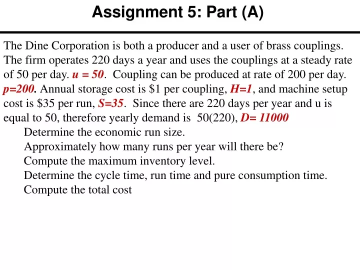
Assignment 5: Part (A) • The Dine Corporation is both a producer and a user of brass couplings. The firm operates 220 days a year and uses the couplings at a steady rate of 50 per day. u = 50. Coupling can be produced at rate of 200 per day. p=200. Annual storage cost is $1 per coupling, H=1, and machine setup cost is $35 per run, S=35. Since there are 220 days per year and u is equal to 50, therefore yearly demand is 50(220), D= 11000 • Determine the economic run size. • Approximately how many runs per year will there be? • Compute the maximum inventory level. • Determine the cycle time, run time and pure consumption time. • Compute the total cost
EPQ: One period and One year p-u u One Period One Year
Imax, Ordering Cost and Carrying Cost I max I max I max I max
The Problem • The Dine Corporation is both a producer and a user of brass couplings. The firm operates 220 days a year and uses the couplings at a steady rate of 50 per day. u = 50. Coupling can be produced at rate of 200 per day. p=200. Annual storage cost is $1 per coupling, H=1, and machine setup cost is $35 per run, S=35. Since there are 220 days per year and u is equal to 50, therefore yearly demand is 50(220), D= 11000 • Determine the economic run size. • Approximately how many runs per year will there be? • Compute the maximum inventory level. • Determine the cycle time, run time and pure consumption time. • Compute the total cost
EPQ and # of Runs • u =50, p=200, H=1, S=35, D= 11000 • Determine the economic run size. • Approximately how many runs per year will there be? • D/Q = 11000/1013 = 10.85
Run Time I max p-u u d2 d1 How much do we produce each time? Q How long does it take to produce Q? d1 What is our production rate per day? p • Run Time? • Q = pd1 1013 = 200d1 • d1= 1013/200 = 5.0
Maximum Inventory I max p-u u d2 d1 • Maximum Inventory ? • At what rate inventory is accumulated? • p-u • For how long? • d1 • What is the maximum inventory? • IMax • IMax = (p-u)d1 • IMax = (200-50)(5.06) = 759
Pure Consumption Time I max p-u u d2 d1 • What is the Maximum inventory? • IMax • How long does it take to consume IMax ? • d2 • At which rate Imax is consumed for d2 days • u • Imax = ud2 • 759 = 50d2 • d2 = 15.18
Cycle Time, Total Cost • Cycle Time ? • d1 + d2 = 5.06 + 15.18 = 20.24 • Total Cost ? • TC = H(IMax/2) + S(D/Q) • TC = 1(759/2) + 35 (11000/1013) • TC = 379.5 + 379.5 = 759
Assignment4: Part (B) (a) : If average demand per day is 20 units and lead time is 10 days. Assuming zero safety stock. ss=0, compute ROP? (b): If average demand per day is 20 units and lead time is 10 days. Assuming 70 units of safety stock. SS=70, compute ROP? (c) : If average demand during the lead time is 200 and standard deviation of demand during lead time is 25. Compute ROP at 90% service level. Compute ss (d) : If average demand per day is 20 units and standard deviation of demand is 5 per day, and lead time is 16 days. Compute ROP at 90% service level. Compute ss (e) : If demand per day is 20 units and lead time is 16 days and standard deviation of lead time is 4 days. Compute ROP at 90% service level. Compute ss
Demand Forecast, and LeadTimes Re-Order Point (ROP) in periodic inventory control is the beginning of each period. (ROP) in perpetual inventory control is the inventory level equal to the demand during the lead timeplus a safety stock to cover demand variability. Lead Time is the time interval from placing an order until receiving the order. If there were no variations in demand, and demand was really constant; the ss is zero and ROP is when inventory on hand is equal to the average demand during lead time.
ROP; Fixed d, Fixed LT, Zero SS (a) :If average demand per day is 20 units and lead time is 10 days. Assuming zero safety stock. ss = 0 What is ROP? ROP = demand during lead time + ss ROP = demand during lead time Demand during lead time = (lead time) × (demand per unit of time) Demand during lead time = 20 × 10 = 200
ROP; Fixed d, Fixed LT, Positive SS Problem 4(b):If average demand per day is 20 units and lead time is 10 days. Assuming 70 units of safety stock. ss = 70 What is ROP ROP = demand during lead time + ss Demand during lead time = 200 ss = 70 ROP = 200+70 = 270
Safety Stock and ROP Risk of a stockout Average demand Safety stock z-scale Service level Probability of no stockout ROP Quantity 0 z Each Normal variable x is associated with a standard Normal Variable z x is Normal (Average x , Standard Deviation x) z is Normal (0,1) • There is a table for z which tells us • Given anyprobability of not exceeding z. What is the value of z • Given anyvalue forz. What is the probability of not exceeding z
Common z Values Service level Risk of a stockout Probability of no stockout ROP Quantity Average demand Safety stock 0 z z-scale Risk Service level z value .1 .9 1.28 .05 .95 1.65 .01 .99 2.33
Relationship between z and Normal Variable x Service level Risk of a stockout Probability of no stockout ROP Quantity Average demand Safety stock 0 z z-scale z = (x-Average x)/(Standard Deviation of x) x = Average x +z (Standard Deviation of x) μ = Average x σ = Standard Deviation of x Risk Service z value level .1 .9 1.28 .05 .95 1.65 .01 .99 2.33 x = μ +z σ
Relationship between z and Normal Variable ROP Service level Risk of a stockout Probability of no stockout ROP Quantity Average demand Safety stock 0 z z-scale LTD = Lead Time Demand ROP = Average LTD +z (Standard Deviation of LTD) ROP = Average LTD +ss ss = z (Standard Deviation of LTD)
Safety Stock and ROP Service level Risk of a stockout Probability of no stockout ROP Quantity Average demand Safety stock 0 z z-scale Risk Service level z value .1 .9 1.28 .05 .95 1.65 .01 .99 2.33 ss = z × (standard deviation of demand during lead time)
ROP; total demand during lead time is variable Service level Risk of a stockout Probability of no stockout ROP Expected demand Safety stock x • (c) : If average demand during the lead time is 200 and standard deviation of demand during lead time is 25. • Compute ROP at 90% service level. • Compute SS
ROP; total demand during lead time is variable Service level Risk of a stockout Probability of no stockout z Risk Service level z value .1 .9 1.28 .05 .95 1.65 .01 .99 2.33
ROP; total demand during lead time is variable z = 1.28 z = (X- μ)/σ X= μ +z σ μ = 200 σ = 25 X= 200+ 1.28 × 25 X= 200 + 32 ROP = 232 SS = 32
ROP; Variable d, Fixed LT • (d) :If average demand per day is 20 units and standard deviation of demand is 5 per day, and lead time is 16 days. • Compute ROP at 90% service level. • Compute SS
ROP; Variable d, Fixed LT • Previous Problem • If average demand during the lead time is 200 and standard deviation of demand during lead time is 25. • Compute ROP at 90% service level. • Compute SS • This Problem • If average demand per day is 20 units and standard deviation of demand is 5 per day, and lead time is 16 days. • Compute ROP at 90% service level. • Compute SS If we can transform this problem into the previous problem, then we are done, because we already know how to solve the previous problem.
ROP; Variable d, Fixed LT • If average demand per day is 20 units and standard deviation of demand is 5 per day, and lead time is 16 days. • Compute ROP at 90% service level. • Compute SS • What is the average demand during the lead time • What is standard deviation of demand during lead time
Demand During Lead Time If demand is variable and Lead time is fixed
Now it is transformed into our previous problem where total demand during lead time is variable • The average demand during the lead time is 320 and the standard deviation of demand during the lead time is 20. • Compute ROP at 90% service level. • Compute SS Service level Risk of a stockout Probability of no stockout ROP Expected demand Safety stock x
ROP; Variable d, Fixed LT z = 1.28 z = (X- μ)/σ X= μ +z σ μ = 320 σ = 20 X= 320+ 1.28 × 20 X= 320 + 25.6 X= 320 + 26 ROP = 346 SS = 26
Demand Fixed, Lead Time variable If lead time is variable and demand is fixed
Lead Time Variable, Demand fixed e) Demand of sand is fixed and is 50 tons per week. The average lead time is 2 weeks. Standard deviation of lead time is .5 week. Assuming that the management is willing to accept a risk no more that 10%. Compute ROP and SS. Acceptable risk; 10% z = 1.28