Download
1 / 35
350 likes | 434 Views
Profile methods for homolog identification. Overview. What are profiles? How are profiles related to MSAs? How are profiles used? How does sequence selection affect profile performance? Profile drift Sequence weighting

E N D
Overview • What are profiles? • How are profiles related to MSAs? • How are profiles used? • How does sequence selection affect profile performance? • Profile drift • Sequence weighting • Generalization techniques to derive effective amino acid distributions • BLOSUM62, Dirichlet mixture densities, etc • PSI-BLAST homology clustering • FlowerPower homology clustering • SCI-PHY subfamily identification
Seq1 M V V S - - P Seq2 M V V S T G P Seq3 M V V S S G P Seq4 M V L S S P P Seq5 M - L S G P P HMM construction using an initial multiple sequence alignment Delete/skip Insert Match
D S I F M K D S V F M K D T I W M K D T I W M K D T V W M K Profile or HMM parameter estimation using small training sets What other amino acids might be seen at this position among homologs? What are their probabilities? .
In searching for family members, all features must be assumed to be equally informative.
Without knowing which features are more important, would we recognize this relative?
Gathering family members allows us to identify conserved attributes and create a profile Conserved: stripes, cat. Variable: coat color, size.
Profile construction allows us to identify sometruly remote relatives
D S I F M K D S V F M K D T I W M K D T I W L K D T L W L R The context is critical when estimating amino acid distributions This position may be critical for function or structure, and may not allow substitutions .
ˆ pi = the estimated probability of amino acid ‘i’ n = (n1,…,n20) = the count vector summarizing the observed amino acids at a position. j = (j,1 ,…, j,20 ) = the parameters of component j of the Dirichlet mixture . Combining Prior Knowledge with Observations using Dirichlet Mixture Densities “Dirichlet Mixtures: A Method for Improved Detection of Weak but Significant Protein Sequence Homology” Sjölander, Karplus, Brown, Hughey, Krogh, Mian and Haussler. CABIOS (1996)
ˆ pi = the estimated probability of amino acid ‘i’ n = (n1,…,n20) = the count vector summarizing the observed amino acids at a position. j = (j,1 ,…, j,20 ) = the parameters of component j of the Dirichlet mixture . Combining Prior Knowledge with Observations using Dirichlet Mixture Densities Sjölander, Karplus, Brown, Hughey, Krogh, Mian and Haussler (1996) “Dirichlet Mixtures: A Method for Improved Detection of Weak but Significant Protein Sequence Homology.” CABIOS
Parameters estimated using Expectation Maximization (EM) algorithm. Training data: 86,000 columns from BLOCKS alignment database.
Experimental Validation Of all methods (of estimating amino acid distributions in profiles) tested, Dirichlet mixture priors produced the fewest false positives (FP) and false negatives (FN) in discrimination tests. Benchmark dataset of biologically curated proteins. Cutoff chosen when |FP| = |FN|, to balance specificity and sensitivity. Detection of conserved segments in proteins: Iterative scanning of sequence databases with alignment blocks. Tatusov, Altschul and Koonin, 1994 Proc. National Academy of Sciences 91: 12091-12095
Dirichlet mixture densities(a short list of publications using) • Profile/HMM construction (homolog detection and protein fold prediction) • Brown, Hughey, Krogh, Mian, Sjölander, Haussler. (1993) “Using Dirichlet mixture priors to derive hidden Markov models for protein families.” Proc Int Conf Intell Syst Mol Biol. (The first publication of the method, at the ISMB meeting.) • Sjölander et al (1996) “Dirichlet mixtures: a method for improving detection of weak but significant protein sequence homology” CABIOS (CABIOS became the journal Bioinformatics.) • Tatusov, Altschul and Koonin (1994). “Detection of conserved segments in proteins: Iterative scanning of sequence databases with alignment blocks” PNAS. (Compared different methods for constructing profiles for iterated sequence search. The use of Dirichlet mixture densities produced the fewest FP and FN in database search. ) • Karplus et al (1997), “Predicting protein structure using hidden Markov models” Proteins, Structure Function and Genetics. (Invited paper based on results of the CASP2 protein structure prediction experiment; the UCSC-EBI group placed among the top in the world, using HMMs constructed using Dirichlet mixture densities. ) • Park et al. 1998 “Sequence comparisons using multiple sequences detect three times as many remote homologues as pairwise methods.” JMB (The SAM-T98 HMM method (using Dirichlet mixture densities) was the top performer in a heated competition between BLAST, PSI-BLAST, ISS, and T2K.) • Brown, Krishnamurthy, Dale, Christopher, Sjolander. “Subfamily HMMs in functional genomics”. PSB. Dirichlet mixture densities used to weight shared amino acids across subfamilies • Subfamily identification • Sjölander (1998) “Phylogenetic inference in protein superfamilies: analysis of SH2 domains” ISMB. (The initial publication of the SCI-PHY algorithm (then called “Bayesian Evolutionary Tree Estimation), using Dirichlet mixture densities to cut a tree into subtrees to identify subfamilies.) • Motif detection • Bailey and Elkan (1995) “The value of prior knowledge in discovering motifs with MEME” Proc. ISMB
FlowerPowerStep 1: Construct set of candidate homologs using PSI-BLAST Q=query Q
Step 2: Select and align core set. • Inclusion criteria: • Significant E-value (length-dependent) • Bi-directional alignment overlap (ensures hits align along entire length to query and vice versa) Q MUSCLE multiple alignment (Edgar, 2003)
Step 3: Run SCI-PHY to identify subfamilies and build subfamily HMMs (SHMMs) Q Brown, Krishnamurthy & Sjölander, "Automated Protein Subfamily Identification and Classification," PLoS Computational Biology 2007
Step 4: SHMMs compete for sequences from SearchDB. Sequences meeting criteria are aligned to their closest SHMM. Q
Step 5: Run SCI-PHY on extended alignment to identify new subfamilies and construct SHMMs. Q
Comparing FlowerPower, BLAST, PSI-BLAST and UCSC T2KTest: Clustering global homologs Agreement at domain structure determined by PFAM. SCOP used to cluster PFAM domains into structural equivalence classes.
A B B A C C A C B Subfamily identification accuracy relies on knowledge (or prediction) of specificity determinants • Major differences between phylogenies for protein superfamilies occur at the coarse branching order (near the root) • Knowing which positions are functionally important is required for phylogenetic tree topology accuracy • Errors in coarse branching order can cause errors in phylogenomic inference of function Src homology 2 (SH2) domain 1SPSA "Phylogenetic inference in protein superfamilies: Analysis of SH2 domains," Sjölander, ISMB 1998
Seq1 LERY-K Seq2 LDRFPR Seq3 IERYGK Seq4 MDRF-K Seq5 VERYGK 5 3 1 4 2 Phylogenetic tree & subfamily decomposition Multiple sequence alignment Subfamily Classification In PHYlogenomics (SCI-PHY) Agglomerative clustering Input: MSA Initialize: construct profile1 for each row in MSA While (#clusters > 1) { Join closest2 pair of clusters Re-estimate profile1 Compute encoding cost3 for this stage } /* cut tree using minimum encoding cost */ Use Dirichlet mixture densities Distance function: relative entropy Detection of critical positions
Cost N 1 # classes Subfamilies identified using minimum encoding cost principles • Each stage of the algorithm defines a different set of alignments, one for each cluster (“subfamily”). • Find the point during the clustering where the encoding cost of the alignments is minimal. This defines the subfamily decomposition. N= number of sequences. S= number of subfamilies; n c,1…n c,s are the amino acids aligned by subfamilies 1 through s at column c. represents the Dirichlet mixture prior.
Validation Datasets • SCOP-PFAM515 • 515 PFAM full MSAs, selected such that no two were drawn from the same SCOP fold, and each produced >=2 SCI-PHY subfamilies • Used in testing • homolog recognition (comparing subfamily vs family HMMs) • subfamily HMM-based classification • SCI-PHY agreement with conserved clades in phylogenetic trees • EC • 57 PFAM families; a subset of SCOP-PFAM515 such that each contained >=2 EC numbers • Used in testing subfamily identification methods for ability to reproduce functional subtypes • EXPERT • 5 superfamilies, with 8 overall classification schemes • From SFLD, GPCRDb and NucleaRDB • Used in testing subfamily identification methods for ability to reproduce functional subtypes
A SCI-PHY occasionally provides a refinement of the same functional subtype based on taxonomic groupings (e.g., vertebrate vs invertebrate, as shown here) • Other SCI-PHY subfamilies can contain paralogs (typically corresponding to the same function, but potentially different tissue/temporal expression) • PhyloFacts book bpg000014 (Voltage-gated K+ Shaker/Shaw)
Results on EC dataset Distances between predicted subtypes and expert classification: Edit distance (#split/merge operations needed); penalizes over-refinement more than heterogeneity VI (variation of information) distance: penalizes differences in large classes more than in smaller Purity: the fraction of subfamilies predicted containing members of only one subtype
3 4 5 1 2 6 7 • At completely conserved positions, and subfamily gapped positions: Use match state distributions estimated for general (family) HMM. • At other positions: • Estimate Dirichlet mixture density posterior for each subfamily at each position separately. • Use Dirichlet density posteriors to weight contributions from other subfamilies. • Compute amino acid distribution using weighted counts and standard Dirichlet procedure. Subfamily HMM construction Error Brown et al,“Subfamily HMMs in functional genomics” (2005) Pacific Symposium on Biocomputing
Subfamily HMMs increase the separation between true and false positives • 515 unique SCOP folds • PFAM full MSAs • Family HMMs constructed using SAM w0.5 software • Scored against Astral PDB90 At an e-value cutoff of 10e-20, SHMMs detected 73% of SCOP superfamily members, whereas family HMMs detected only 31%.