Download
1 / 27
320 likes | 642 Views
Compiler Optimization and Code Generation. Professor: Sc.D., Professor Vazgen Melikyan. Course Overview. Introduction: Overview of Optimizations 1 lecture Intermediate-Code Generation 2 lectures Machine-Independent Optimizations 3 lectures Code Generation 2 lectures.

E N D
Compiler Optimization and Code Generation Professor: Sc.D., Professor Vazgen Melikyan
Course Overview • Introduction: Overview of Optimizations • 1 lecture • Intermediate-Code Generation • 2 lectures • Machine-Independent Optimizations • 3 lectures • Code Generation • 2 lectures
The Function of Compilers • Translate program in one language to executable program in other language. • Typically lower abstraction level • E.g., convert C++ into ( x86, SPARC, HP PA, IBM PPC) object code • Optimize the Code • E.g., make the code run faster (transforms a computation to an equivalent but better form ) • Difference between optimizing and non-optimizing compiler ~ 4x ( Proebsting’s law ) • “Optimize” is a bit of a misnomer, the result is not actually optimal
The Structure of a Compiler Source Code ( C, C++, Java, Verilog ) Lexical analyzer Syntax analyzer Semantic analyzer Symbol-table Error handler Intermediate Code Generator Machine-Independent Code Optimizer Code generator Machine-Dependent Code Optimizer Target Machine Code ( Alpha, SPARC, x86, IA-64 )
The Structure of a Compiler:Work Example position = initial + rate*60 Intermediate Code Generator Lexical analyzer t1 = inttofloat (60) t2 = id3 * t1 t3 = id2 + t2 id1 = t3 <id,1> <=> <id,2><+><id,3><*><60> Syntax analyzer Code Optimizer = t1 = id3 * 60.0 id1 = id2 + t1 + <id,1> * <id,2> 60 <id,3> Semantic analyzer Code generator = LDF R2, id3 MULF R2, R2, #60.0 LDF R1, id2 ADDF R1, R1, R2 STF id1, R1 + <id,1> * <id,2> inttoflat <id,3> 60
Lexical Analyzer • The first phase of a compiler is called lexical analysis or scanning. • The lexical analyzer reads the stream of characters making up the source program and groups the characters into meaningful sequences called lexemes. • For each lexeme, the lexical analyzer produces as output a token of the form: • token-name - abstract symbol that is used during syntax analysis. • attribute-value - points to an entry in the symbol table for this token. Information from the symbol-table entry is needed for semantic analysis and code generation. <token-name, attribute-value>
Syntax Analyzer: Parser • The second phase of the compiler is syntax analysis or parsing. • The parser uses the first components of the tokens produced by the lexical analyzer to create a tree-like intermediate representation that depicts the grammatical structure of the token stream. • A typical representation is a syntax tree in which each interior node represents an operation and the children of the node represent the arguments of the operation.
Semantic Analyzer • The semantic analyzer uses the syntax tree and the information in the symbol table to check the source program for semantic consistency with the language definition. • Gathers type information and saves it in either the syntax tree or the symbol table, for subsequent use during intermediate-code generation. • An important part of semantic analysis is type checking, where the compiler checks that each operator has matching operands.
How Compiler Improves Performance Execution time = Operation count * Machine cycles per operation • Minimize the number of operations • Arithmetic operations, memory accesses • Replace expensive operations with simpler ones • E.g., replace 4-cycle multiplication with1-cycle shift • Minimize cache misses • Both data and instruction accesses • Perform work in parallel • Instruction scheduling within a thread • Parallel execution across multiple threads
Global Steps of Optimization • Formulate optimization problem: • Identify opportunities of optimization • Representation: • Control-flow graph • Control-dependence graph • Def/use, use/def chains • SSA (Static Single Assignment) • Analysis: • Control-flow • Data-flow • Code Transformation • Experimental Evaluation (and repeat process)
Other Optimization Goals Besides Performance • Minimizing power and energy consumption • Finding (and minimizing the impact of ) software bugs • Security vulnerabilities • Subtle interactions between parallel threads • Increasing reliability, fault-tolerance
Types of Optimizations • Peephole • Local • Global • Loop • Interprocedural, whole-program or link-time • Machine code • Data-flow • SSA-based • Code generator • Functional language
Other Optimizations • Bounds-checking elimination • Dead code elimination • Inline expansion or macro expansion • Jump threading • Macro compression • Reduction of cache collisions • Stack height reduction
Basic Blocks • Basic blocks are maximal sequences of consecutive three-address instructions. • The flow of control can only enter the basic block through the first instruction in the block. (no jumps into the middle of the block ) • Control will leave the block without halting or branching, except possibly at the last instruction in the block. • The basic blocks become the nodes of a flow graph, whose edges indicate which blocks can follow which other blocks.
Partitioning Three-address Instructions into Basic Blocks 4 • Input: A sequence of three-address instructions • Output: A list of the basic blocks for that sequence in which each instruction is assigned to exactly one basic block • Method: Determine instructions in the intermediate code that are leaders: the first instructions in some basic block (instruction just past the end of the intermediate program is not included as a leader) • The rules for finding leaders are: • The first three-address instruction in the intermediate code • Any instruction that is the target of a conditional or unconditional jump • Any instruction that immediately follows a conditional or unconditional jump
Partitioning Three-address Instructions into Basic Blocks: Example • i = 1 • j = 1 • t1 = 10 * i • t2 = t1 + j • j = j + 1 • if j <= 10 goto (3) • i = i + 1 • if i <= 10 goto (2) • i = 1 • t3 = i – 1 • if i <= 10 goto (10) • First, instruction 1 is a leader by rule (1). Jumps are at instructions 6, 8, and 11. By rule (2), the targets of these jumps are leaders ( instructions 3, 2, and 10, respectively) • By rule (3), each instruction following a jump is a leader; instructions 7 and 9. • Leaders are instructions 1, 2, 3, 7, 9 and 10. The basic block of each leader contains all the instructions from itself until just before the next leader.
Flow Graphs • Flow Graph is the representation of control flow between basic blocks. The nodes of the flow graph are the basic blocks. • There is an edge from block B to block C if and only if it is possible for the first instruction in block C to immediately follow the last instruction in block B. There are two ways that such an edge could be justified: • There is a conditional or unconditional jump from the end of B to the beginning of C. • C immediately follows B in the original order of the three-address instructions, and B does not end in an unconditional jump. • B is a predecessor of C, and C is a successor of B.
Flow Graphs: Example Flow Graph Example of program in Example(1). The block led by first statement of the program is the start, or entrynode. • Entry • Exit • B1: i = 1 • B6: t3 = i – 1 • if i <= 10 goto (10) • B2: j = 1 • B3: t1 = 10 * i • t2 = t1 + j • j = j + 1 • if j <= 10 goto (3) • B5: i = 1 • B4: i = i + 1 • if i <= 10 goto (2)
Flow Graphs: Representation • Flow graphs, being quite ordinary graphs, can be represented by any of the data structures appropriate for graphs. • The content of a node (basic block) might be represented by a pointer to the leader in the array of three-address instructions, together with a count of the number of instructions or a second pointer to the last instruction. • Since the number of instructions may be changed in a basic block frequently, it is likely to be more efficient to create a linked list of instructions for each basic block.
Local Optimizations • Analysis and transformation performed within a basic block • No control flow information is considered • Examples of local optimizations: • Local common sub expression elimination analysis: same expression evaluated more than once in b. transformation: replace with single calculation • Local constant folding or elimination analysis: expression can be evaluated at compile time transformation: replace by constant, compile-time value • Dead code elimination
Global Optimizations: Intraprocedural • Global versions of local optimizations • Global common sub-expression elimination • Global constant propagation • Dead code elimination • Loop optimizations • Reduce code to be executed in each iteration • Code motion • Induction variable elimination • Other control structures • Code hoisting: eliminates copies of identical code on parallel paths in a flow graph to reduce code size.
Induction Variable Elimination • Intuitively • Loop indices are induction variables (counting iterations) • Linear functions of the loop indices are also induction variables (for accessing arrays) • Analysis: detection of induction variable • Optimizations • Strength reduction: replace multiplication by additions • Elimination of loop index: replace termination by tests on other induction variables
Loop Invariant Code Motion • Analysis • A computation is done within a loop and result of the computation is the same as long as keep going around the loop • Transformation • Move the computation outside the loop a = b + c t = b + c a = t
Loop Fusion (1) • Loop fusion, also called loop jamming, is a compiler optimization, a loop transformation, which replaces multiple loops with a single one. Original Loop inti, a[100], b[100]; for (i = 0; i < 100; i++) { a[i] = 1; } for (i = 0; i < 100; i++) { b[i] = 2; } After Loop Fusion inti, a[100], b[100]; for (i = 0; i < 100; i++) { a[i] = 1; b[i] = 2; }
Loop Fusion (2) • Loop fission(or loop distribution) is a compiler optimization technique attempting to break a loop into multiple loops over the same index range but each taking only a part of the loop's body. • The goal is to break down large loop body into smaller ones to achieve better utilization of locality of reference. It is the reverse action to loop fusion. This optimization is most efficient in multi-core processors that can split a task into multiple tasks for each processor. Original Loop inti, a[100], b[100]; for (i = 0; i < 100; i++) { a[i] = 1; b[i] = 2; } After Loop Fission inti, a[100], b[100]; for (i = 0; i < 100; i++) { a[i] = 1; } for (i = 0; i < 100; i++) { b[i] = 2; }