Download
1 / 29
310 likes | 529 Views
Eigenstructure Methods for Noise Covariance Estimation. Olawoye Oyeyele AICIP Group Presentation April 29th, 2003. Outline. Background Adaptive Antenna Arrays Array Signal Processing Discussion Next Steps. Objective. Discuss Antenna Arrays and similarities to sensor arrays

E N D
Eigenstructure Methods for Noise Covariance Estimation Olawoye Oyeyele AICIP Group Presentation April 29th, 2003
Outline • Background • Adaptive Antenna Arrays • Array Signal Processing • Discussion • Next Steps
Objective • Discuss Antenna Arrays and similarities to sensor arrays • Investigate methods used for covariance estimation in adaptive antenna arrays with a focus on applicable eigenstructure methods
Background • Antenna Arrays are a group of antenna elements with signal processing capability which enables the dynamic update of the beam pattern • Various elemental configurations possible: • Linear • Circular • Planar • Major objective is to cancel interference • Sensor Arrays are similar to antenna arrays
… d 0 1 3 … k-2 k-1 Uniformly spaced Linear Array Signals arriving at the (K-1)th element lag those at the (k-2)th element but lead in time . . . … ..
Adaptive Antenna Array Generally, complex weights are used.
Basic Antenna Array Parameters Array Propagation Vector: contains the information on angle of arrival of the signal Array Factor: the radiation pattern of the array consisting of isotropic elements
Steering Vector • Contains the responses of all the vectors of an array. • Used to accomplish electronic Beam Steering – each element of vector performs phase delay with respect to the next. • In electronic steering no physical movement of the array is done. • Mechanical beam steering involves physically moving the elements of the array. • Multiple steering vectors constitute an Array Manifold • Array manifold is an array of steering vectors
Comparison between Sensor and Antenna Arrays *Multipath components are signal waves arriving at different times because each sample traveled varying distances as a result of reflections.
Array Signal Processing • Techniques employed in adaptive antenna arrays • They include: • Beamforming(Adaptive & Partially Adaptive) • Direction of Arrival Estimation(DOA) • These techniques require the estimation of covariance matrices
Beamforming • Adjusting signal amplitudes and phases to form a desired beam • Estimation of signal arriving from a desired direction in the presence of noise by exploiting the spatial separation of the source of the signals. • Applicable to radiation and reception of energy. • May be classified as: • Data Independent • Statistically optimum • Adaptive • Partially Adaptive
Adaptive Beamforming • Can be performed in both frequency and time domains • Sample Matrix Inversion • Least Mean Squares(LMS) • Recursive Least Squares(RLS) • Neural Network
Two-Element Example Desired Array Output: Interference arrives at angle of pi/6 w1 w2 Received Interference signals: To completely cancel interference (yd=y) the following weights must be used: w1=1/2-j/2; w2=1/2+j/2 y
Eigenstructure Technique • For L x L matrix • Largest M eigenvalues correspond to M directional sources • L-M smallest eigenvalues represent the background noise power • Eigenvectors are orthogonal – may be thought of as spanning L-dimensional space
Eigenstructure Technique • The space spanned by eigenvectors may be partitioned into two subspaces • Signal subspace • Noise subspace • The steering vectors corresponding to the directional sources are orthogonal to the noise subspace • noise subspace is orthogonal to signal subspace thus steering vectors are contained in the signal subspace • When explicit correlation matrix is required it may be estimated from the samples.
Sample Matrix Inversion(SMI) • Operates directly on the snapshot of data to estimate covariance matrix Weight Vector can be estimated as:
SMI Disadvantages • Increased computational complexity • Inversion of large matrices and numerical instability due to roundoff errors
Recursive Least Squares(RLS) where is the forgetting factor – ensures that data in the previous data are forgotten Thus, the matrix is found recursively
Recursive Least Squares(RLS) • Fast convergence even with large eigenvalue spread. • Recursively updates estimates
Direction of Arrival Estimation(DOA) • DOA involves computing the spatial spectrum and determining the maximas. • Maximas correspond to DOAs • Typical DOA algorithms include: • Multiple SIgnal Classification(MUSIC) • Estimation of Signal Parameters via Rotational Invariance Techniques(ESPRIT) • Spectral Estimation • Minimum Variance Distortionless Response(MVDR) • Linear Prediction • Maximum Likelihood Method(MLM) • MUSIC is explored in this presentation
MUSIC Algorithm • Useful for estimating • Number of sources • Strength of cross-correlation between source signals • Directions of Arrival • Strength of noise • Assumes number of sources < Number of antenna elements. • else signals may be poorly resolved • Estimates noise subspace from available samples
MUSIC algorithm-contd Thus, Assumes that noise at each array element is additive white and gaussian(AWGN) uncorrelated between elements with the same variance and that arriving signals have a mean of zero.
MUSIC Algorithm-contd • After computing the eigenvalues of Ruu,the eigenvalues of ARssAH can be computing by subtracting the variances as follows: • If number of incident signals D, is less than number of number of antenna elements M, then M-D eigenvalues are zero.
Spatial Spectrum 2 signals, 8 array elements
Discussion • Signal should lie mostly in subspace spanned by eigenvectors associated with large eigenvalues - noise is weak in this subspace. • Idea of communicating where noise is weak similar to other spectrum optimization problems – e.g. water-filling solution to communication spectrum allocation problem • Signal strength is maximum in subspace where noise is weak
Next steps • Apply to the Restricted Matched Filter problem- select a fixed subset of sensors in a cluster • Obtain results that demonstrate the optimality of the Receiver operating characteristic
References • Lal C. Godara, "Application of Antenna Arrays to Mobile Communications, Part I: Performance Improvements, Feasibility and System Considerations," Proc. of the IEEE, Vol. 85, No 7, pp. 1031- 1060, July 1997. • Lal C. Godara, "Application of Antenna Arrays to Mobile Communications, Part II: Beamforming and Direction of Arrival Considerations," Proc. of the IEEE, Vol. 85, No 8, pp. 1195- 1245, July 1997. • B.D. Van Veen and K. M. Buckley "Beamforming: A versatile Approach to Spatial Filtering" IEEE ASSP Magazine, pp. 4-24, April 1988. • John Litva and Titus Kwok-Yeung Lo, Digital Beamforming in wireless communications, Artech House Publishers, 1996.