Download
1 / 14
140 likes | 237 Views
The Finite-Volume Dynamical Core on GPUs within GEOS-5. William Putman Global Modeling and Assimilation Office NASA GSFC. Outline. Development Platform. Motivation Test advection kernel Approach in GEOS-5 Design for FV development Early results Status/future.

E N D
The Finite-Volume Dynamical Core on GPUs within GEOS-5 William Putman Global Modeling and Assimilation Office NASA GSFC Programming weather, climate, and earth-system models on heterogeneous multi-core platforms- Boulder, CO
Outline Development Platform • Motivation • Test advection kernel • Approach in GEOS-5 • Design for FV development • Early results • Status/future • NASA Center for Climate Simulation • GPU Cluster • 32 Compute Nodes • 2 Hex-core 2.8 GHz Intel Xeon Westmere Processors • 48 GB of memory per node • 2 NVidia M2070 GPUs • dedicated x16 PCIe Gen2 connection • Infiniband QDR Interconnect • 64 Graphical Processing Units • 1 Tesla GPU (M2070) • 448 CUDA cores • ECC Memory • 6 GB of GDDR5 memory • 515 Gflop/s of double precision floating point performance (peak) • 1.03 Tflop/s of single precision floating point performance (peak) • 148 GB/sec memory bandwidth • 1 PCIe x16 Gen2 system interface http://www.nccs.nasa.gov/gpu_front.html
PDF of Average Convective Cluster Brightness Temperature Motivation Global Cloud Resolving GEOS-6 • We are pushing the resolution of global models into the 10- to 1-km range • GEOS-5 can fit a 5-day forecast at 10-km within the 3-hour window required for operations using 12,000 Intel Westmere cores • At current cloud-permitting resolutions (10- to 3-km) required scaling of 300,000 cores is reasonable (though not readily available) • To get to global cloud resolving (1-km or finer) requires order 10-million cores • Weak scaling of cloud-permitting GEOS-5 model indicates need for accelerators • ~90% of those computations are in the dynamics 3.5-km GEOS-5 Simulated Clouds
Motivation Idealized FV advection kernel • The ultimate target: the FV dynamical core – accounts for ~ 90% of the compute cycles at high-resolution (1- to 10-km) • The D-grid Shallow water routines are as costly as the non-hydrostatic dynamics (thus first pieces to attack) • An offline Cuda C demonstration kernel was developed for the 2-D advection scheme • For a 512x512 domain, the benchmark revealed up to 80x speedup • Caveats: Written entirely on the GPU (no data transfers) • Single CPU to Single GPU speedup • compares Cuda C to C code Data Transfers from Host to the Device cost about 10-15% Fermi GPGPU 16x 32-core Streaming Multiprocessors CUDA Profiler – Used to profile
Motivation Idealized FV advection kernel - tuning Fermi GPGPU 16x 32-core Streaming Multiprocessors • The Finite-Volume kernel performs 2-dimensional advection on a 256x256 mesh • Blocks on the GPU are used to decompose the mesh in a similar fashion to MPI domain decomposition • Optimal distribution of blocks improve occupancy on the GPU • Targeting 100% Occupancy and threads in multiples of the Warp size (32) • Best performance with 16, 32 or 64 threads in the Y-direction Fermi – Compute 2.0 CUDA device: [Tesla M2050] Occupancy - the amount of shared memory and registers used by each thread block, or the ratio of active warps to the maximum number of warps available Warp – A collection of 32 threads CUDA Profiler – Used to profile and compute occupancy Total Number of Threads
Approach GEOS-5 Modeling Framework and the FV3 dycore • Earth System Modeling Framework (ESMF) • GEOS-5 uses a fine-grain component design with light-weight ESMF components used down to the parameterization level • A hierarchical topology is used to create Composite Components, defining coupling (relations) between parents and children components • As a result, implementation of GEOS-5 residing entirely on GPUs is unrealistic, we must have data exchanges to the CPU for ESMF component connections • PGI Cuda Fortran – CPU and GPU code co-exist in the same code-base (#ifdef _CUDA) • Flexible Modeling System (FMS) • Component based modeling framework developed and implemented at GFDL • The MPP layer provides a uniform interface to different message-passing libraries, used for all MPI communication in FV • The GPU implementation of FV will extend out to this layer and exchange data for halo updates between GPU and CPU
Approach Single Precision FV cubed C360 Single Precision C360 Double Precision • FV was converted to single precision prior to beginning GPU development 1.8x - 1.3x Speedup
Approach Domain Decomposition (MPI and GPU) • MPI Decomposition – 2D in X,Y • GPU blocks distributed in X,Y within the decomposed domain
Approach GEOS-5 Modeling Framework and the FV dycore • Bottom-up development • Target kernels for 1D and 2D advection will be developed at the lowest level of FV (tp_core module) • fxppm/fyppm • xtp/ytp • fv_tp_2d • The advection kernels are reused throughout the c_sw and d_sw routines (the Shallow Water equations) • delp/pt/vort advection • At the dyn_core layer halo regions will be exchanged between the host and the device • The device data is centrally located and maintained at a high level (fv_arrays) to maintain object oriented approach(and we can pin this memory as needed) • Test-driven development • Offline test modules have been created to develop GPU kernels for tp_core • Easily used to validate results with the CPU code • Improve development time by avoiding costly rebuilds of full GEOS-5 code-base
π Details of the Implementation The FV advection scheme (PPM) Sub-Grid PPM Distribution Schemes ORD=7 details (4th order and continuous before monotonicity)… The value at the edge is an average of two one-sided 2nd order extrapolations across edge discontinuities Directionally split Positivity for tracers 1D flux-form operators • Fitting by Cubic Polynomial to find the value on the other edge of the cell • vanishing 2nd derivative • local mean = cell mean of left/right cells Cross-stream inner-operators
Details of the Implementation Serial offline test kernel for 2D advection (fv_tp_2d with PGI Cuda Fortran) GPU Code istat = cudaMemcpy(q_device, q, NX*NY) call copy_corners_dev<<<dimGrid,dimBlock>>>() call xtp_dev<<<dimGrid,dimBlock>>>() call intermediateQj_dev<<<dimGrid,dimBlock>>>() call ytp_dev<<<dimGrid,dimBlock>>>() call copy_corners_dev<<<dimGrid,dimBlock>>>() call ytp_dev<<<dimGrid,dimBlock>>>() call intermediateQi_dev<<<dimGrid,dimBlock>>>() call xtp_dev<<<dimGrid,dimBlock>>>() call yflux_average_dev<<<dimGrid,dimBlock>>>() call xflux_average_dev<<<dimGrid,dimBlock>>>() istat = cudaMemcpy(fy, fy_device, NX*NY) istat = cudaMemcpy(fx, fx_device, NX*NY) ! Compare fy/fx bit-wise reproducible to CPU code
Details of the Implementation Serial offline test kernel for 2D advection (fv_tp_2d with PGI Cuda Fortran) GPU Code istat = cudaMemcpyAsync(qj_device, q, NX*NY, stream(2)) istat = cudaMemcpyAsync(qi_device, q, NX*NY, stream(1)) call copy_corners_dev<<<dimGrid,dimBlock,0,stream(2)>>>() call xtp_dev<<<dimGrid,dimBlock,0,stream(2)>>>() call intermediateQj_dev<<<dimGrid,dimBlock,0,stream(2)>>>() call ytp_dev<<<dimGrid,dimBlock,0,stream(2)>>>() call copy_corners_dev<<<dimGrid,dimBlock,0,stream(1)>>>() call ytp_dev<<<dimGrid,dimBlock,0,stream(1)>>>() call intermediateQi_dev<<<dimGrid,dimBlock,0,stream(1)>>>() call xtp_dev<<<dimGrid,dimBlock,0,stream(1)>>>() call yflux_average_dev<<<dimGrid,dimBlock,0,stream(2)>>>() call xflux_average_dev<<<dimGrid,dimBlock,0,stream(1)>>>() istat = cudaMemcpyAsync(fy, fy_device, NX*NY, stream(2)) istat = cudaMemcpyAsync(fx, fx_device, NX*NY, stream(1)) Data is copied back to the host for export, but the GPU work can continue…
Speedup Details of the Implementation D_SW – Asynchronous multi-stream 6 GPUs: 6 cores 16.2x 6 GPUs : 36 cores 4.6x 36 GPUs : 36 cores 10.2x CPU Time GPU Time GPU Code 6 cores D_SW 75.5365 36 cores D_SW 21.5692 6 GPUs D_SW 4.6509 36 GPUs D_SW 2.1141 call getCourantNumbersY(…stream(2)) call getCourantNumbersX(…stream(1)) call fv_tp_2d(delp…) call update_delp(delp,fx,fy,…) call update_KE_Y(…stream(2)) call update_KE_X(…stream(1)) call divergence_damping() call compute_vorticity() call fv_tp_2d(vort…) call update_uv(u,v,fx,fy,…) istat = cudaStreamSynchronize(stream(2)) istat = cudaStreamSynchronize(stream(1)) istat = cudaMemcpy(delp, delp_dev, NX*NY) istat = cudaMemcpy( u, u_dev, NX*(NY+1)) istat = cudaMemcpy( v, v_dev, (NX+1)*NY) Times for a 1-day 28-km Shallow Water Test Case
Status - Summary • Most of D_SW is implemented on GPU • Preliminary results are being generated (but need to be studied more) • C_SW routine is similar to D_SW, but has not been touched yet • Data transfers between host and device are done asynchronously when possible • Most data transfers will move up to the dyn_core level as implementation progresses, improving performance • Higher-level operations in dyn_core will be tested with pragmas (Kerr - GFDL) • Non-hydrostatic core must be tackled (column based) • Strong scaling potential?