Download
1 / 40
400 likes | 402 Views
Explore the basic principles of population genetics, including X-linked genes and modeling selection. Learn about deviations from Hardy-Weinberg equilibrium (HWE) due to mutation, migration, selection, and drift.

E N D
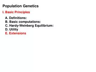
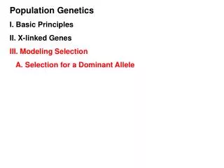
Population Genetics I. Basic Principles II. X-linked Genes III. Modeling Selection IV. OTHER DEVIATIONS FROM HWE
Deviations from HWE I. Mutation A. Basics:
Deviations from HWE I. Mutation A. Basics: 1. Consider a population with: f(A) = p = .6 f(a) = q = .4
Deviations from HWE I. Mutation A. Basics: 1. Consider a population with: f(A) = p = .6 f(a) = q = .4 2. Suppose 'a' mutates to 'A' at a realistic rate of: μ = 1 x 10⁻⁵
Deviations from HWE I. Mutation A. Basics: 1. Consider a population with: f(A) = p = .6 f(a) = q = .4 2. Suppose 'a' mutates to 'A' at a realistic rate of: μ = 1 x 10⁻⁵ 3. Well, what fraction of alleles will change? 'a' will decline by: qm = .4 x 0.00001 = 0.000004 'A' will increase by the same amount.
Deviations from HWE I. Mutation A. Basics: 1. Consider a population with: f(A) = p = .6 f(a) = q = .4 2. Suppose 'a' mutates to 'A' at a realistic rate of: μ = 1 x 10⁻⁵ 3. Well, what fraction of alleles will change? 'a' will decline by: qm = .4 x 0.00001 = 0.000004 'A' will increase by the same amount. 4. So, the new gene frequencies will be: p1 = p + μq = .600004 q1 = q - μq = q(1-μ) = .399996
Deviations from HWE I. Mutation A. Basics: 4. So, the new gene frequencies will be: p1 = p + μq = 1 - q + μq = 1- q(1-μ) = .600004 q1 = q - μq = q(1-μ) = .399996 5. How about with both FORWARD and backward mutation? Δq = νp - μq
Deviations from HWE I. Mutation A. Basics: 4. So, the new gene frequencies will be: p1 = p + μq = 1 - q + μq = 1- q(1-μ) = .600004 q1 = q - μq = q(1-μ) = .399996 5. How about with both FORWARD and backward mutation? Δq = νp - μq - so, if A -> a =v = 0.00008 and a-> = μ = 0.00001, and p = 0.6 and q = 0.4, then:
Deviations from HWE I. Mutation A. Basics: 4. So, the new gene frequencies will be: p1 = p + μq = 1 - q + μq = 1- q(1-μ) = .600004 q1 = q - μq = q(1-μ) = .399996 5. How about with both FORWARD and backward mutation? Δq = νp - μq - so, if A -> a =v = 0.00008 and a->A = μ = 0.00001, and p = 0.6 and q = 0.4, then: Δq = νp - μq = 0.000048 - 0.000004 = 0.000044 q1 = .4 + 0.000044 = 0.400044
Deviations from HWE I. Mutation A. Basics: 4. So, the new gene frequencies will be: p1 = p + μq = 1 - q + μq = 1- q(1-μ) = .600004 q1 = q - μq = q(1-μ) = .399996 5. How about with both FORWARD and backward mutation? - and qeq = v/ v + μ
Deviations from HWE I. Mutation A. Basics: 4. So, the new gene frequencies will be: p1 = p + μq = 1 - q + μq = 1- q(1-μ) = .600004 q1 = q - μq = q(1-μ) = .399996 5. How about with both FORWARD and backward mutation? - and qeq = v/ v + μ = 0.00008/0.00009 = 0.89
Deviations from HWE I. Mutation A. Basics: 4. So, the new gene frequencies will be: p1 = p + μq = 1 - q + μq = 1- q(1-μ) = .600004 q1 = q - μq = q(1-μ) = .399996 5. How about with both FORWARD and backward mutation? - and qeq = v/ v + μ = 0.00008/0.00009 = 0.89 - Δq = (.11)(0.00008) - (.89)(0.00001) = 0.0..... check.
Deviations from HWE I. Mutation A. Basics: B. Other Considerations:
Deviations from HWE I. Mutation A. Basics: B. Other Considerations: - Selection: Selection can BALANCE mutation... so a deleterious allele might not accumulate as rapidly as mutation would predict, because it it eliminated from the population by selection each generation. We'll model these effects later.
Deviations from HWE I. Mutation A. Basics: B. Other Considerations: - Selection: Selection can BALANCE mutation... so a deleterious allele might not accumulate as rapidly as mutation would predict, because it it eliminated from the population by selection each generation. We'll model these effects later. - Drift: The probability that a new allele (produced by mutation) becomes fixed (q = 1.0) in a population = 1/2N (basically, it's frequency in that population of diploids). In a small population, this chance becomes measureable and likely. So, NEUTRAL mutations have a reasonable change of becoming fixed in small populations... and then replaced by new mutations.
Deviations from HWE I. Mutation II. Migration A. Basics: - Consider two populations: p2 = 0.7 q2 = 0.3 p1 = 0.2 q1 = 0.8
Deviations from HWE I. Mutation II. Migration A. Basics: - Consider two populations: p2 = 0.7 q2 = 0.3 p1 = 0.2 q1 = 0.8 suppose migrants immigrate at a rate such that the new immigrants represent 10% of the new population
Deviations from HWE I. Mutation II. Migration A. Basics: - Consider two populations: p2 = 0.7 q2 = 0.3 p1 = 0.2 q1 = 0.8 suppose migrants immigrate at a rate such that the new immigrants represent 10% of the new population
Deviations from HWE I. Mutation II. Migration A. Basics: - Consider two populations: p2 = 0.7 q2 = 0.3 p1 = 0.2 q1 = 0.8 suppose migrants immigrate at a rate such that the new immigrants represent 10% of the new population p(new) = p1(1-m) + p2(m)
Deviations from HWE I. Mutation II. Migration A. Basics: - Consider two populations: p2 = 0.7 q2 = 0.3 p1 = 0.2 q1 = 0.8 suppose migrants immigrate at a rate such that the new immigrants represent 10% of the new population p(new) = p1(1-m) + p2(m) p(new) = 0.2(0.9) + 0.7(0.1) = 0.25
Deviations from HWE I. Mutation II. Migration A. Basics: B. Advanced: - Consider three populations: p1 = 0.7 q1 = 0.3 p2 = 0.2 q2 = 0.8 p3 = 0.6 q3 = 0.4
Deviations from HWE I. Mutation II. Migration A. Basics: B. Advanced: - Consider three populations: - How different are they, genetically? (this can give us a handle on how much migration there may be between them...) p1 = 0.7 q1 = 0.3 p2 = 0.2 q2 = 0.8 p3 = 0.6 q3 = 0.4
Deviations from HWE I. Mutation II. Migration A. Basics: B. Advanced: - Consider three populations: - How different are they, genetically? (this can give us a handle on how much migration there may be between them...) - Compute Nei's Genetic distance: D = -ln [ ∑pi1pi2/ √ ∑pi12 ∑pi22] p1 = 0.7 q1 = 0.3 p2 = 0.2 q2 = 0.8 p3 = 0.6 q3 = 0.4
Deviations from HWE I. Mutation II. Migration A. Basics: B. Advanced: - Consider three populations: - How different are they, genetically? (this can give us a handle on how much migration there may be between them...) - Compute Nei's Genetic distance: D = -ln [ ∑pi1pi2/ √ ∑pi12 ∑pi22] - So, for Population 1 and 2: - ∑pi1pi2 = (0.7*0.2) + (0.3*0.8) = 0.38 - denominator = √ (.49+.09) * (.04+.64) = 0.628 D12 = -ln (0.38/0.62) = 0.50 p1 = 0.7 q1 = 0.3 p2 = 0.2 q2 = 0.8 p3 = 0.6 q3 = 0.4
- Compute Nei's Genetic distance: D = -ln [ ∑pi1pi2/ √ ∑pi12 ∑pi22] - So, for Population 1 and 2: - ∑pi1pi2 = (0.7*0.2) + (0.3*0.8) = 0.38 - denominator = √ (.49+.09) * (.04+.64) = 0.628 D12 = -ln (0.38/0.628) = 0.50 - For Population 1 and 3: - ∑pi1pi2 = (0.7*0.6) + (0.3*0.4) = 0.54 - denominator = √ (.49+.09) * (.36+.16) = 0.55 D13 = -ln (0.54/0.55) = 0.02 - For Population 2 and 3: - ∑pi1pi2 = (0.2*0.6) + (0.8*0.4) = 0.44 - denominator = √ (.04+.64) * (.36+.16) = 0.61 D23 = -ln (0.44/0.61) = 0.33 p1 = 0.7 q1 = 0.3 p2 = 0.2 q2 = 0.8 p3 = 0.6 q3 = 0.4
Deviations from HWE I. Mutation II. Migration III. Non-Random Mating A. Positive Assortative Mating "like phenotype mates with like phenotype"
Deviations from HWE I. Mutation II. Migration III. Non-Random Mating A. Positive Assortative Mating "like phenotype mates with like phenotype" 1. Pattern:
1. Pattern: 2. Effect: - reduction in heterozygosity at this locus; increase in homozygosity.
Deviations from HWE I. Mutation II. Migration III. Non-Random Mating A. Positive Assortative Mating B. Inbreeding 1. Overview:
B. Inbreeding 1. Overview: - Autozygous - inherited alleles common by descent - F = inbreeding coefficient = prob. of autozygosity - so, (1-F) = prob. of allozygosity
B. Inbreeding 1. Overview: - Autozygous - inherited alleles common by descent - F = inbreeding coefficient = prob. of autozygosity - so, (1-F) = prob. of allozygosity - SO: f(AA) = p2(1-F) + p2(F) = D f(Aa) = 2pq(1-F) = H (observed) f(aa) = q2(1-F) + q2(F) = R
B. Inbreeding 1. Overview: - Autozygous - inherited alleles common by descent - F = inbreeding coefficient = prob. of autozygosity - so, (1-F) = prob. of allozygosity - SO: f(AA) = p2(1-F) + p2(F) = D f(Aa) = 2pq(1-F) = H (observed) f(aa) = q2(1-F) + q2(F) = R - SO!! the net effect is a decrease in heterozygosity at a factor of (1-F) each generation. - So, the fractional demise of heterozygosity compared to HWE expectations is also a direct measure of inbreeding! F = (2pq - H)/2pq = (Hexp - Hobs)/ Hexp When this is done on multiple loci, the values should all be similar (as inbreeding affects the whole genotype).
B. Inbreeding 1. Overview: - Example: F = (2pq - H)/2pq = (Hexp - Hobs)/ Hexp p = .5, q = .5, expected HWE heterozygosity = 2pq = 0.5 OBSERVED in F1 = 0.3... so F = (.5 - .3)/.5 = 0.4
Deviations from HWE I. Mutation II. Migration III. Non-Random Mating A. Positive Assortative Mating B. Inbreeding 1. Overview: 2. Effects:
Deviations from HWE I. Mutation II. Migration III. Non-Random Mating A. Positive Assortative Mating B. Inbreeding 1. Overview: 2. Effects: - reduce heterozygosity across entire genome
Deviations from HWE I. Mutation II. Migration III. Non-Random Mating A. Positive Assortative Mating B. Inbreeding 1. Overview: 2. Effects: - reduce heterozygosity across entire genome - rate dependent upon degree of relatedness
Deviations from HWE I. Mutation II. Migration III. Non-Random Mating A. Positive Assortative Mating B. Inbreeding 1. Overview: 2. Effects: - reduce heterozygosity across entire genome - rate dependent upon degree of relatedness - change in genotypic frequencies but no change in gene frequencies as a result of non-random mating ALONE....
Deviations from HWE I. Mutation II. Migration III. Non-Random Mating A. Positive Assortative Mating B. Inbreeding 1. Overview: 2. Effects: - reduce heterozygosity across entire genome - rate dependent upon degree of relatedness - change in genotypic frequencies but no change in gene frequencies as a result of non-random mating ALONE.... - BUT... increasing homozygosity may reveal deleterious recessives.
Deviations from HWE I. Mutation II. Migration III. Non-Random Mating A. Positive Assortative Mating B. Inbreeding 1. Overview: 2. Effects: - reduce heterozygosity across entire genome - rate dependent upon degree of relatedness - change in genotypic frequencies but no change in gene frequencies as a result of non-random mating ALONE.... - BUT... increasing homozygosity may reveal deleterious recessives. - these will be quickly selected against....?
Deviations from HWE I. Mutation II. Migration III. Non-Random Mating A. Positive Assortative Mating B. Inbreeding 1. Overview: 2. Effects: - reduce heterozygosity across entire genome - rate dependent upon degree of relatedness - change in genotypic frequencies but no change in gene frequencies as a result of non-random mating ALONE.... - BUT... increasing homozygosity may reveal deleterious recessives. - these will be quickly selected against, but that reduces fecundity (inbreeding depression) and reduces genetic variation.