Download
1 / 68
700 likes | 706 Views
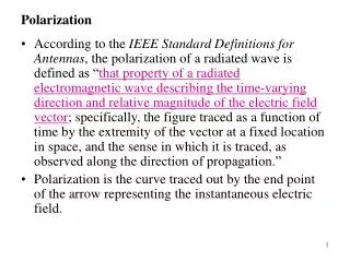
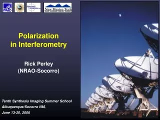
Polarization in Interferometry. Steven T. Myers (NRAO-Socorro). Polarization in interferometry. Astrophysics of Polarization Physics of Polarization Antenna Response to Polarization Interferometer Response to Polarization Polarization Calibration & Observational Strategies

E N D
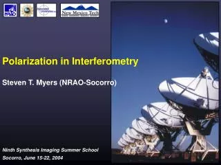
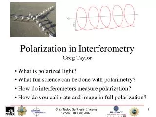
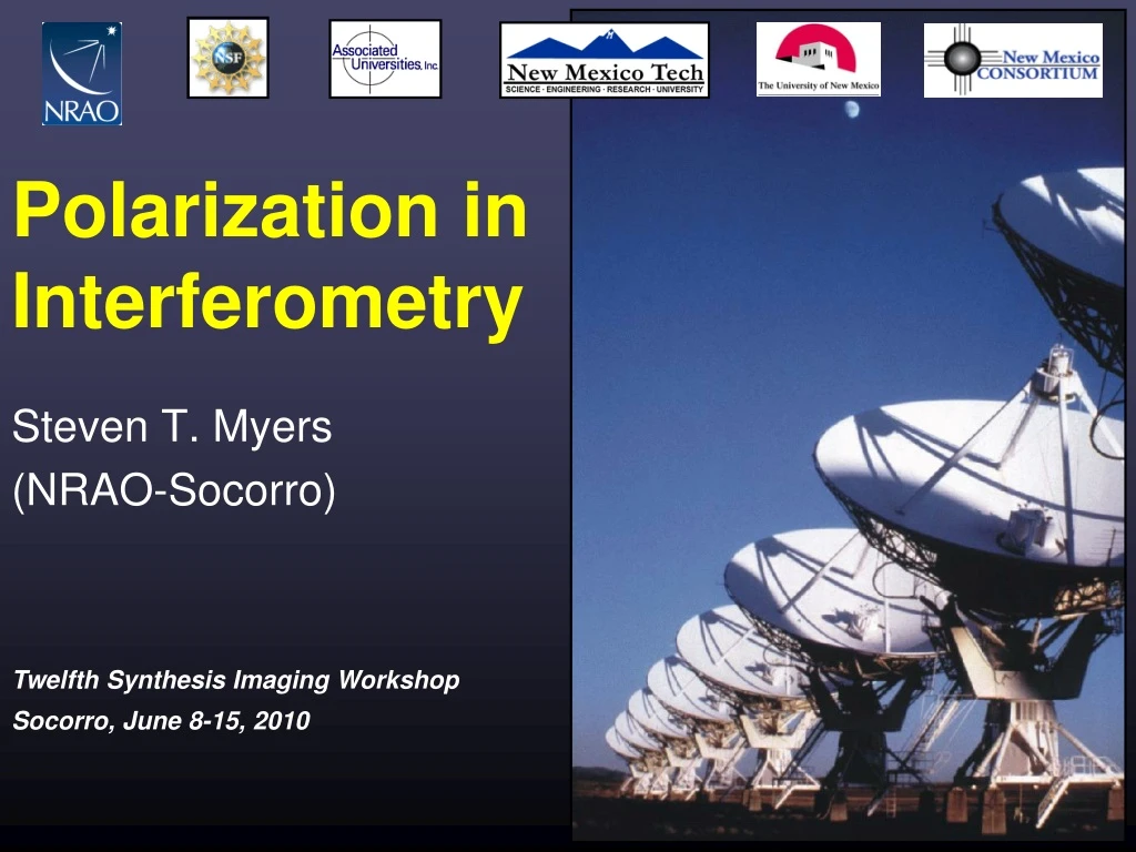
Polarization in Interferometry Steven T. Myers (NRAO-Socorro)
Polarization in interferometry • Astrophysics of Polarization • Physics of Polarization • Antenna Response to Polarization • Interferometer Response to Polarization • Polarization Calibration & Observational Strategies • Polarization Data & Image Analysis S.T. Myers – Twelfth Synthesis Imaging Workshop, June 8, 2010
DON’T PANIC! • There are lots of equations and concepts. Hang in there. • I will illustrate the concepts with figures and ‘handwaving’. • Many good references: • Synthesis Imaging II: Lecture 6, also parts of 1, 3, 5, 32 • Born and Wolf: Principle of Optics, Chapters 1 and 10 • Rolfs and Wilson: Tools of Radio Astronomy, Chapter 2 • Thompson, Moran and Swenson: Interferometry and Synthesis in Radio Astronomy, Chapter 4 • Tinbergen: Astronomical Polarimetry. All Chapters. • J.P. Hamaker et al., A&A, 117, 137 (1996) and series of papers • Great care must be taken in studying these references – conventions vary between them. S.T. Myers – Twelfth Synthesis Imaging Workshop, June 8, 2010
Polarization Astrophysics S.T. Myers – Twelfth Synthesis Imaging Workshop, June 8, 2010
Why Measure Polarization? • Electromagnetic waves are intrinsically polarized • monochromatic waves are fully polarized • Polarization state of radiation can tell us about: • the origin of the radiation • intrinsic polarization, orientation of generating B-field • the medium through which it traverses • propagation and scattering effects • unfortunately, also about the purity of our optics • you may be forced to observe polarization even if you do not want to! S.T. Myers – Twelfth Synthesis Imaging Workshop, June 8, 2010
Astrophysical Polarization • Examples: • Processes which generate polarized radiation: • Synchrotron emission: Up to ~80% linearly polarized, with no circular polarization. Measurement provides information on strength and orientation of magnetic fields, level of turbulence. • Zeeman line splitting: Presence of B-field splits RCP and LCP components of spectral lines (2.8 Hz/mG for HI). Measurement provides direct measure of B-field. • Processes which modify polarization state: • Free electron scattering: Induces a linear polarization which can indicate the origin of the scattered radiation. • Faraday rotation: Magnetoionic region rotates plane of linear polarization. Measurement of rotation gives B-field estimate. • Faraday conversion: Particles in magnetic fields can cause the polarization ellipticity to change, turning a fraction of the linear polarization into circular (possibly seen in cores of AGN) S.T. Myers – Twelfth Synthesis Imaging Workshop, June 8, 2010
Example: Radio Galaxy 3C31 3 kpc • VLA @ 8.4 GHz • Laing (1996) • Synchrotron radiation • relativistic plasma • jet from central “engine” • from pc to kpc scales • feeding >10kpc “lobes” • E-vectors • along core of jet • radial to jet at edge S.T. Myers – Twelfth Synthesis Imaging Workshop, June 8, 2010
Example: Radio Galaxy Cygnus A 10 kpc • VLA @ 8.5 GHz B-vectors Perley & Carilli (1996) S.T. Myers – Twelfth Synthesis Imaging Workshop, June 8, 2010
Example: Faraday rotation of CygA • See review of “Cluster Magnetic Fields” by Carilli & Taylor 2002 (ARAA) S.T. Myers – Twelfth Synthesis Imaging Workshop, June 8, 2010
Example: Zeeman effect S.T. Myers – Twelfth Synthesis Imaging Workshop, June 8, 2010
Example: the ISM of M51 • Trace magnetic field structure in galaxies • follow spiral structure • origin? • amplified in dynamo? Neininger (1992) S.T. Myers – Twelfth Synthesis Imaging Workshop, June 8, 2010
Scattering • Anisotropic Scattering induces Linear Polarization • electron scattering (e.g. in Cosmic Microwave Background) • dust scattering (e.g. in the millimeter-wave spectrum) Planck predictions – Hu & Dodelson ARAA 2002 Animations from Wayne Hu S.T. Myers – Twelfth Synthesis Imaging Workshop, June 8, 2010
Polarization Fundamentals S.T. Myers – Twelfth Synthesis Imaging Workshop, June 8, 2010
The Polarization Ellipse • From Maxwell’s equations E•B=0 (E and B perpendicular) • By convention, we consider the time behavior of the E-field in a fixed perpendicular plane, from the point of view of the receiver. • For a monochromatic wave of frequency n, we write • These two equations describe an ellipse in the (x-y) plane. • The ellipse is described fully by three parameters: • AX, AY, and the phase difference, d = fY-fX. transverse wave S.T. Myers – Twelfth Synthesis Imaging Workshop, June 8, 2010
Elliptically Polarized Monochromatic Wave • The simplest description • of wave polarization is in • a Cartesian coordinate • frame. • In general, three parameters are needed to describe the ellipse. • If the E-vector is rotating: • clockwise, wave is ‘Left Elliptically Polarized’, • counterclockwise, is ‘Right Elliptically Polarized’. • The angle a = atan(AY/AX) is used later … equivalent to 2 independent Ex and Ey oscillators S.T. Myers – Twelfth Synthesis Imaging Workshop, June 8, 2010
Polarization Ellipse Ellipticity and P.A. • A more natural description is in a frame (x,h), rotated so the x-axis lies along the major axis of the ellipse. • The three parameters of the ellipse are then: Ah : the major axis length tan c = Ax/Ah: the axial ratio • : the major axis p.a. • The ellipticity c is signed: c > 0 REP c < 0 LEP • = 0,90° Linear (d=0°,180°) • = ±45° Circular (d=±90°) S.T. Myers – Twelfth Synthesis Imaging Workshop, June 8, 2010
Circular Basis • We can decompose the E-field into a circular basis, rather than a (linear) Cartesian one: • where AR and AL are the amplitudes of two counter-rotating unit vectors, eR (rotating counter-clockwise), and eL (clockwise) • NOTE: R,L are obtained from X,Y by d=±90° phase shift • It is straightforward to show that: S.T. Myers – Twelfth Synthesis Imaging Workshop, June 8, 2010
Circular Basis Example • The black ellipse can be decomposed into an x-component of amplitude 2, and a y-component of amplitude 1 which lags by ¼ turn. • It can alternatively be decomposed into a counterclockwise rotating vector of length 1.5 (red), and a clockwise rotating vector of length 0.5 (blue). S.T. Myers – Twelfth Synthesis Imaging Workshop, June 8, 2010
The Poincare Sphere • Treat 2y and 2c as longitude and latitude on sphere of radius A=E2 Rohlfs & Wilson S.T. Myers – Twelfth Synthesis Imaging Workshop, June 8, 2010
Stokes parameters • Spherical coordinates: radius I, axes Q, U, V • I = EX2 + EY2 = ER2 + EL2 • Q = I cos 2c cos 2y = EX2 - EY2 = 2 ERELcos dRL • U = I cos 2c sin 2y = 2 EXEYcos dXY = 2 ERELsin dRL • V = I sin 2c = 2 EXEYsin dXY = ER2 - EL2 • Only 3 independent parameters: • wave polarization confined to surface of Poincare sphere • I2 = Q2 + U2 + V2 • Stokes parameters I,Q,U,V • defined by George Stokes (1852) • form complete description of wave polarization • NOTE: above true for 100% polarized monochromatic wave! S.T. Myers – Twelfth Synthesis Imaging Workshop, June 8, 2010
Linear Polarization • Linearly Polarized Radiation: V = 0 • Linearly polarized flux: • Q and U define the linear polarization position angle: • Signs of Q and U: Q > 0 U > 0 U < 0 Q < 0 Q < 0 U > 0 U < 0 Q > 0 S.T. Myers – Twelfth Synthesis Imaging Workshop, June 8, 2010
Simple Examples • If V = 0, the wave is linearly polarized. Then, • If U = 0, and Q positive, then the wave is vertically polarized, Y=0° • If U = 0, and Q negative, the wave is horizontally polarized, Y=90° • If Q = 0, and U positive, the wave is polarized at Y = 45° • If Q = 0, and U negative, the wave is polarized at Y = -45°. S.T. Myers – Twelfth Synthesis Imaging Workshop, June 8, 2010
Illustrative Example: Non-thermal Emission from Jupiter • Apr 1999 VLA 5 GHz data • D-config resolution is 14” • Jupiter emits thermal radiation from atmosphere, plus polarized synchrotron radiation from particles in its magnetic field • Shown is the I image (intensity) with polarization vectors rotated by 90° (to show B-vectors) and polarized intensity (blue contours) • The polarization vectors trace Jupiter’s dipole • Polarized intensity linked to the Io plasma torus S.T. Myers – Twelfth Synthesis Imaging Workshop, June 8, 2010
Why Use Stokes Parameters? • Tradition • They are scalar quantities, independent of basis XY, RL • They have units of power (flux density when calibrated) • They are simply related to actual antenna measurements. • They easily accommodate the notion of partial polarization of non-monochromatic signals. • We can (as I will show) make images of the I, Q, U, and V intensities directly from measurements made from an interferometer. • These I,Q,U, and V images can then be combined to make images of the linear, circular, or elliptical characteristics of the radiation. S.T. Myers – Twelfth Synthesis Imaging Workshop, June 8, 2010
Partial Polarization • Monochromatic radiation is a myth. • No such entity can exist (although it can be closely approximated). • In real life, radiation has a finite bandwidth. • Real astronomical emission processes arise from randomly placed, independently oscillating emitters (electrons). • We observe the summed electric field, using instruments of finite bandwidth. • Despite the chaos, polarization still exists, but is not complete – partial polarization is the rule. S.T. Myers – Twelfth Synthesis Imaging Workshop, June 8, 2010
Stokes Parameters for Partial Polarization Stokes parameters defined in terms of mean quantities: Note that now, unlike monochromatic radiation, the radiation is not necessarily 100% polarized. S.T. Myers – Twelfth Synthesis Imaging Workshop, June 8, 2010
Summary – Fundamentals • Monochromatic waves are polarized • Expressible as 2 orthogonal independent transverse waves • elliptical cross-section polarization ellipse • 3 independent parameters • choice of basis, e.g. linear or circular • Poincare sphere convenient representation • Stokes parameters I, Q, U, V • I intensity; Q,U linear polarization, V circular polarization • Quasi-monochromatic “waves” in reality • can be partially polarized • still represented by Stokes parameters S.T. Myers – Twelfth Synthesis Imaging Workshop, June 8, 2010
Antenna Polarization S.T. Myers – Twelfth Synthesis Imaging Workshop, June 8, 2010
Measuring Polarization on the sky • Coordinate system dependence: • I independent • V depends on choice of “handedness” • V > 0 for RCP • Q,U depend on choice of “North” (plus handedness) • Q “points” North, U 45 toward East • Polarization Angle Y Y = ½ tan-1 (U/Q) (North through East) • also called the “electric vector position angle” (EVPA) • by convention, traces E-field vector (e.g. for synchrotron) • B-vector is perpendicular to this Q U S.T. Myers – Twelfth Synthesis Imaging Workshop, June 8, 2010
Optics – Cassegrain radio telescope • Paraboloid illuminated by feedhorn: Feeds arranged in focal plane (off-axis) S.T. Myers – Twelfth Synthesis Imaging Workshop, June 8, 2010
Optics – telescope response • Reflections • turn RCP LCP • E-field (currents) allowed only in plane of surface • “Field distribution” on aperture for E and B planes: Cross-polarization at 45° No cross-polarization on axes S.T. Myers – Twelfth Synthesis Imaging Workshop, June 8, 2010
Example – simulated VLA patterns • EVLA Memo 58 “Using Grasp8 to Study the VLA Beam” W. Brisken Linear Polarization Circular Polarization cuts in R & L S.T. Myers – Twelfth Synthesis Imaging Workshop, June 8, 2010
Example – measured VLA patterns • AIPS Memo 86 “Widefield Polarization Correction of VLA Snapshot Images at 1.4 GHz” W. Cotton (1994) Circular Polarization Linear Polarization S.T. Myers – Twelfth Synthesis Imaging Workshop, June 8, 2010
Polarization Reciever Outputs • To do polarimetry (measure the polarization state of the EM wave), the antenna must have two outputs which respond differently to the incoming elliptically polarized wave. • It would be most convenient if these two outputs are proportional to either: • The two linear orthogonal Cartesian components, (EX, EY) as in ATCA and ALMA • The two circular orthogonal components, (ER, EL) as in VLA • Sadly, this is not the case in general. • In general, each port is elliptically polarized, with its own polarization ellipse, with its p.a. and ellipticity. • However, as long as these are different, polarimetry can be done. S.T. Myers – Twelfth Synthesis Imaging Workshop, June 8, 2010
Polarizers: Quadrature Hybrids • We’ve discussed the two bases commonly used to describe polarization. • It is quite easy to transform signals from one to the other, through a real device known as a ‘quadrature hybrid’. • To transform correctly, the phase shifts must be exactly 0 and 90 for all frequencies, and the amplitudes balanced. • Real hybrids are imperfect – generate errors (mixing/leaking) • Other polarizers (e.g. waveguide septum, grids) equivalent 0 X R Four Port Device: 2 port input 2 ports output mixing matrix 90 90 Y L 0 S.T. Myers – Twelfth Synthesis Imaging Workshop, June 8, 2010
Polarization Interferometry S.T. Myers – Twelfth Synthesis Imaging Workshop, June 8, 2010
Four Complex Correlations per Pair • Two antennas, each with two differently polarized outputs, produce four complex correlations. • From these four outputs, we want to make four Stokes Images. Antenna 1 Antenna 2 R1 L1 R2 L2 X X X X RR1R2 RR1L2 RL1R2 RL1L2 S.T. Myers – Twelfth Synthesis Imaging Workshop, June 8, 2010
Outputs: Polarization Vectors • Each telescope receiver has two outputs • should be orthogonal, close to X,Y or R,L • even if single pol output, convenient to consider both possible polarizations (e.g. for leakage) • put into vector S.T. Myers – Twelfth Synthesis Imaging Workshop, June 8, 2010
Correlation products: coherency vector • Coherency vector: outer product of 2 antenna vectors as averaged by correlator • these are essentially the uncalibrated visibilitiesv • circular products RR, RL, LR, LL • linear products XX, XY, YX, YY • need to include corruptions before and after correlation S.T. Myers – Twelfth Synthesis Imaging Workshop, June 8, 2010
Polarization Products: General Case What are all these symbols? vpq is the complex output from the interferometer, for polarizations p and q from antennas 1 and 2, respectively. Y and c are the antenna polarization major axis and ellipticity for states p and q. I,Q, U, and V are the Stokes Visibilities describing the polarization state of the astronomical signal. G is the gain, which falls out in calibration. CONVENTION – WE WILL ABSORB FACTOR ½ INTO GAIN!!!!!!! S.T. Myers – Twelfth Synthesis Imaging Workshop, June 8, 2010
Coherency vector and Stokes vector • Maps (perfect) visibilities to the Stokes vector s • Example: circular polarization (e.g. VLA) • Example: linear polarization (e.g. ALMA, ATCA) S.T. Myers – Twelfth Synthesis Imaging Workshop, June 8, 2010
Corruptions: Jones Matrices • Antenna-based corruptions • pre-correlation polarization-dependent effects act as a matrix muliplication. This is the Jones matrix: • form of J depends on basis (RL or XY) and effect • off-diagonal terms J12 and J21 cause corruption (mixing) • total J is a string of Jones matrices for each effect • Faraday, polarized beam, leakage, parallactic angle S.T. Myers – Twelfth Synthesis Imaging Workshop, June 8, 2010
Parallactic Angle, P • Orientation of sky in telescope’s field of view • Constant for equatorial telescopes • Varies for alt-az telescopes • Rotates the position angle of linearly polarized radiation (R-L phase) • defined per antenna (often same over array) • P modulation can be used to aid in calibration S.T. Myers – Twelfth Synthesis Imaging Workshop, June 8, 2010
Visibilities to Stokes on-sky: RL basis • the (outer) products of the parallactic angle (P) and the Stokes matrices gives • this matrix maps a sky Stokes vector to the coherence vector representing the four perfect (circular) polarization products: Circular Feeds: linear polarization in cross hands, circular in parallel-hands S.T. Myers – Twelfth Synthesis Imaging Workshop, June 8, 2010
Visibilities to Stokes on-sky: XY basis • we have • and for identical parallactic angles f between antennas: Linear Feeds: linear polarization present in all hands circular polarization only in cross-hands S.T. Myers – Twelfth Synthesis Imaging Workshop, June 8, 2010
Basic Interferometry equations • An interferometer naturally measures the transform of the sky intensity in uv-space convolved with aperture • cross-correlation of aperture voltage patterns in uv-plane • its tranform on sky is the primary beamA with FWHM ~ l/D • The “tilde” quantities are Fourier transforms, with convention: S.T. Myers – Twelfth Synthesis Imaging Workshop, June 8, 2010
Polarization Interferometry : Q & U • Parallel-hand & Cross-hand correlations (circular basis) • visibility k (antenna pair ij , time, pointing x, channel n, noise n): • where kernel A is the aperture cross-correlation function, f is the parallactic angle, and Q+iU=P is the complex linear polarization • the phase of P is j (the R-L phase difference) S.T. Myers – Twelfth Synthesis Imaging Workshop, June 8, 2010
Example: RL basis imaging • Parenthetical Note: • can make a pseudo-I image by gridding RR+LL on the Fourier half-plane and inverting to a real image • can make a pseudo-V image by gridding RR-LL on the Fourier half-plane and inverting to real image • can make a pseudo-(Q+iU) image by gridding RL to the full Fourier plane (with LR as the conjugate) and inverting to a complex image • does not require having full polarization RR,RL,LR,LL for every visibility (unlike calibration/correction of visibilities) • More on imaging ( & deconvolution ) tomorrow! S.T. Myers – Twelfth Synthesis Imaging Workshop, June 8, 2010
Polarization Leakage, D • Polarizer is not ideal, so orthogonal polarizations not perfectly isolated • Well-designed systems have d < 1-5% (but some systems >10% ) • A geometric property of the antenna, feed & polarizer design • frequency dependent (e.g. quarter-wave at center n) • direction dependent (in beam) due to antenna • For R,L systems • parallel hands affected as d•Q + d•U , so only important at high dynamic range (because Q,U~d, typically) • cross-hands affected as d•Iso almost always important Leakage of q into p (e.g. L into R) S.T. Myers – Twelfth Synthesis Imaging Workshop, June 8, 2010
Leakage revisited… • Primary on-axis effect is “leakage” of one polarization into the measurement of the other (e.g. R L) • but, direction dependence due to polarization beam! • Customary to factor out on-axis leakage into D and put direction dependence in “beam” • example: expand RL basis with on-axis leakage • similarly for XY basis S.T. Myers – Twelfth Synthesis Imaging Workshop, June 8, 2010