Download
1 / 41
410 likes | 552 Views
The true asymmetry between synoptic cyclone and anticyclone amplitudes: Implications for filtering methods in Lagrangian feature tracking. With David Battisti. Single Winter SLP- departure from global mean .

E N D
The true asymmetry between synoptic cyclone and anticyclone amplitudes: Implications for filtering methods in Lagrangian feature tracking With David Battisti
Over the storm track region, cyclones (lows) have larger magnitude than anticyclones (highs) in the raw data • Does this necessarily imply that cyclones have larger magnitude than anticyclones?
Top Animation is A Traveling Symmetric Wave PLUS A Stationary Low
Bottom Animation is: A Traveling Asymmetric Wave Amplified By A lens (Region of Amplified Waves)
Can we separate these two examples by taking out the time mean? Top Animation: The time mean is the Stationary Feature Bottom Animation: The time mean is the net affect of the asymmetric wave
Are the two different (do we care)? • In the top case, the cyclones and anticyclones have the same magnitude and the observed cyclone growth is not synoptic growth but a reflection of the background state • In the bottom case, the cyclones and anticyclones have a magnitude asymmetry in the wave and the large cyclone magnitude reflect synoptic growth
SLP Cyclone magnitude Wave magnitude or stationary climatolgy? How is this picture affected by the way the “background” is removed? Hoskins and Hodges, 2002
Is this a reasonable question to ask? • Wallace et. al 1988: The differences between cyclones and anticyclones are largely a reflection of background climatology. • Can we separate the waves from the background state?
Outline of talk • I: Different methods of removing “background” field from synoptic fields • II: The affect of background state removal on Lagrangian tracking statistics • III: How much of the climatological mean state is related to synoptic waves
I: Different methods of removing “background” field from synoptic fields • A.) Temporal Filter • Filter the time series at each gridpoint • Does not take into account spatial information • B.) Spatial Filter • Filter the spatial map at each time step • Does not take into account temporal information
Temporal Filter- Time Domain High pass filter with cutoff 1/20 days
Spatially Filtering- Take a raw field at a given time 1030 Instantaneous SLP (hPa) 1020 1010 hPa 1000 990 980
In the spectral domain Cutoff at total wavenumber 5
Resulting filtered small scale field 15 10 5 0 hPa -5 -10 -15
I: Conclusions (thus far) • Spatial and temporal filters allow substantially different information to be included in the synoptic field • Spatially filtered fields retain a component of the time mean field that is comparable in magnitude to typical synoptic disturbances; the temporal filter removes the entire time mean field
How does the choice of filter affect the feature tracking statistics? • Similar question was addressed by Anderson et al. 2002, they found: - Temporal filter gives weak systems with cyclone/anticyclone symmetry - Spatial filter properly determines differences in cyclone and anticyclone tracks and intensity • We will re-address this issue using NCEP reanalysis winter (NDJFM) SLP • The tracking algorithm is that of Hodges, 2001
Colors = Mean Feature Magnitude (hPa) Contours = Number of Features Identified (# per Month) Cyclones hPa Anticyclones hPa
Colors = Cyclone Magnitude – Anticyclone Magnitude (hPa) Contours = Spatially Filtered Time mean (hPa)
Composite Features • In each region, make SLP maps relative to the location of the 100 highest magnitude features of each type ( cyclones and anticyclones defined by spatial and temporal filters • Subtract out climatology
Mid-latitude section Spatially Filtered hPa Temporally Filtered
Northern-latitude section Spatially Filtered hPa Temporally Filtered
Southern-latitude section Spatially Filtered hPa Temporally Filtered
II: Conclusions this section • Inclusion of the time mean SLP field in the spatially filtered fields skews the tracking statistics towards large magnitude cyclones (anticyclones) in the climatological lows (highs); such an asymmetry is a misrepresentation of the synoptic fields • The temporal filter produces a modest cyclone/anticyclone magnitude asymmetry that is consistent with the data
III: How much of the climatological mean state is related to synoptic waves
Eulerian Distribution on the right side Top Panel ------- MODE MEAN Bottom Panel
How can we estimate the net affect of passing waves? • The first three moments of the SLP distribution at each gridpoint uniquely define a skew-normal distribution • The separation of the mean and mode is analytically determined (offset due to skewness)
Partitioning of the NDJFM Mean SLP field hPa Same analysis with filtered fields gives similar results
Conclusions • The spatial filter distorts the synoptic fields in an unphysical way that is unrelated to synoptic waves • The temporal filter produces a modest cyclone/anticyclone magnitude asymmetry consistent with the data • The conclusions reached here for SLP also hold for geopotential at other levels and to a lesser extent for vorticity tracking