Download
1 / 29
290 likes | 304 Views
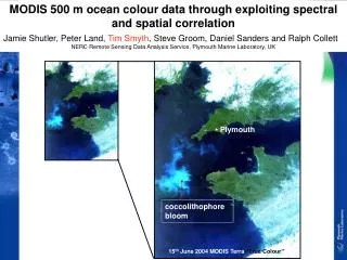
coccolithophore bloom. 15 th June 2004 MODIS Terra “True Colour”. MODIS 500 m ocean colour data through exploiting spectral and spatial correlation. Jamie Shutler, Peter Land, Tim Smyth , Steve Groom, Daniel Sanders and Ralph Collett

E N D
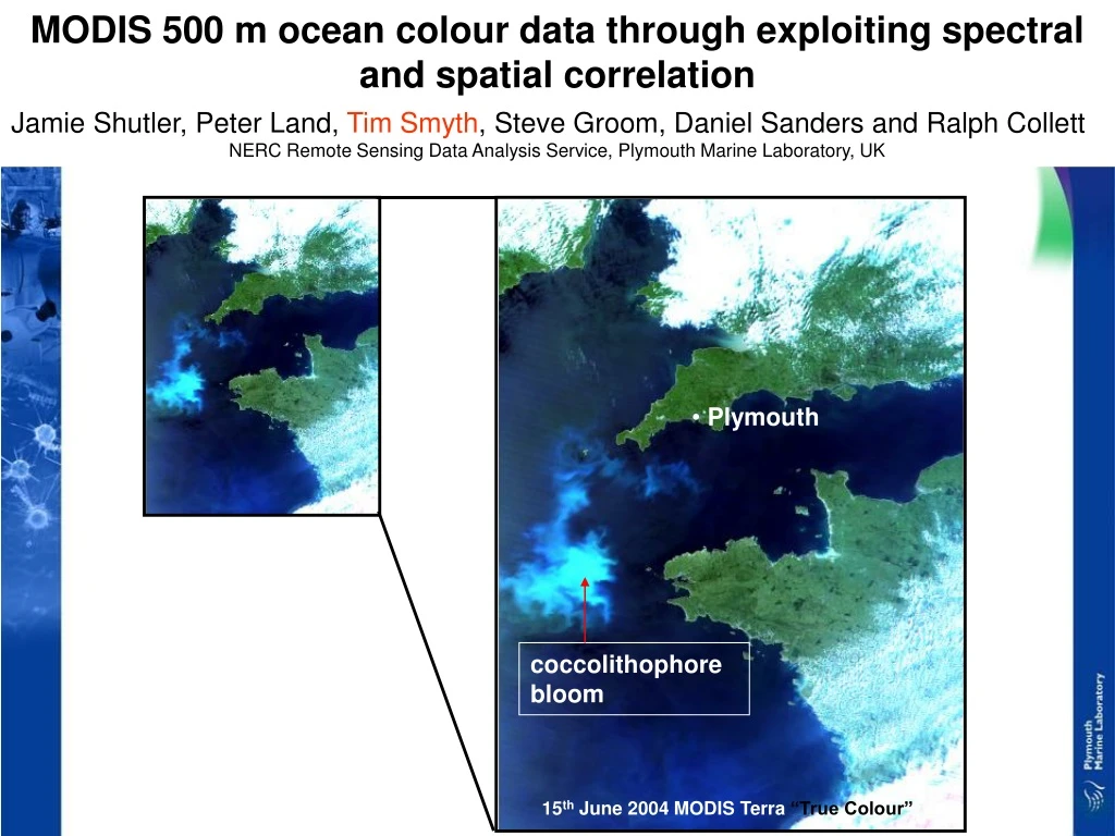
coccolithophore bloom 15th June 2004 MODIS Terra “True Colour” MODIS 500 m ocean colour data through exploiting spectral and spatial correlation Jamie Shutler, Peter Land, Tim Smyth, Steve Groom, Daniel Sanders and Ralph Collett NERC Remote Sensing Data Analysis Service, Plymouth Marine Laboratory, UK • Plymouth
1) What is ocean colour? The need for atmospheric correction 2) The Remote Sensing Data Analysis Service (RSDAS) DB processing chain details 3) Why use MODIS DB data? 4) MODIS 500 m data: Why do we need it? Methodology Results Application Future developments 5) Conclusions Overview
“A term that refers to the spectral dependence of the radiance leaving a water body” (NOAA glossary) Lord Rayleigh (1842-1919): “The much-admired dark blue of the deep sea has nothing to do with the colour of the water, but is simply the blue of the sky seen by reflection.” Raman (1922): “A voyage to Europe in the summer of 1921 gave me the first opportunity of observing the wonderful blue opalescence of the Mediterranean Sea. It seemed not unlikely that the phenomenon owed its origin to the scattering of sunlight by the molecules of the water” 1) What is ocean colour?
1) What is ocean colour? • Mobley (1994): “Natural waters, both fresh and saline, are a witch’s brew of dissolved and particulate matter. These solutes and particles are both optically significant and highly variable in kind and concentration” a(λ) = aw(λ) + aph(λ) + ap(λ) + ay(λ) bb(λ) = bbw(λ) + bbp(λ) • reflectance (R) which can be detected using remote sensing:
CDOM bloom? Sediment Coccolithophores Phytoplankton – fine eddy structure Clear blue ocean
Clouds Clouds 1) What is ocean colour? – the need for atmospheric correction • cloud masking – less rigorous on sensors with no IR bands • Lw – only 5% of signal reaching satellite: rest due to Lp • Lp components: molecular (Rayleigh) & aerosols
1) What is ocean colour? – the need for atmospheric correction • Dark pixel approximation • over oceanic regions assume Lw(765,865) = 0 • any signal due to Lp (765,885) • remove Rayleigh and extrapolate aerosol to other wavelengths
A NERC funded service provided by PML Remote Sensing Group Provides Earth Observation data and information to underpin science in the UK academic community Currently funded primarily for marine science (~20% non marine) Guiding points include: • Timeliness – DB data processing in near-real time • To guide research ships at sea • Increasing input to monitoring systems (e.g. western English Channel andIrish Sea coastal observatories) • see Shutler et al. poster • Ease of use of data by specialists and non specialists alike • Complementarity – we don’t do what ESA or NASA does already 2) The Remote Sensing Data Analysis Service (RSDAS)
2) RSDAS – DB processing chain details NASA /NOAA Centres provide global/backup coverage Password protected Web site with simple Java Image analysis Internet 10 Terabyte Image Database Near-real time Level 2 products ~0.5h AVHRR ~0.5h SeaWiFS ~1h MODIS RSDAS Users Atmospheric correction Internet <100 Mbit/s FTP Navigation Satellite link • Level 2/3 data • Sea-surface temperature • Ocean colour properties • Atmospheric properties • Earth/terrestrial properties Level 0/1 data Received in Plymouth: ~26 passes/day =15GB/day Dundee SatelliteReceiving Station Scientists at sea/ In the field
00:00 Data transfer 00:20 Waiting 00:25 Level 0 – 1b 00:35 Level 2 00:55 Granule stitching and mapping 00:60 Web products 2) RSDAS – DB processing chain details Passes split into 3 granules and processed in parallel on Linux Beowulf cluster
DB data is crucially important to RSDAS – cruise support (285 d yr-1) MODIS provides free-to-air DB ocean colour unlike: MERIS SeaWiFS (licence + user agreement; now data encrypted) Two sensors (Aqua and Terra) - multiple daily passes ameliorate cloud problems MODIS Terra + Aqua: 27 Jan 2004 MODIS Terra: 27 Jan 2004 1131 UTC MODIS Aqua: 27 Jan 2004 1310 UTC + = 3) Why use MODIS DB data? Shutler JD, Smyth TJ, Land PE, Groom SB (2005) A near-real time automatic MODIS data processing system Int. J. Remote Sens. 26 (5): 1049-1055
detail available within estuaries – although still adjacency issues to resolve ii) Water quality – e.g. Harmful Algal Blooms; Eutrophication; pollution HAB May 2000 4) MODIS 500m data - Why do we need it? i) Coastal and large estuarine studies 500 m 1 km
11 July 2005 1338UTC Aqua nLw(469) Turbidity front Physics “mixing up” the biology 4) MODIS 500m data - Why do we need it? iii) Improved spatial resolution of features e.g. eddies, fronts
4) MODIS 500m data - methodology • Aim: Atmospherically corrected 500 m chlorophyll product • simple (Carder 2003) Chl band ratio algorithm 488/551 (1 km) • ideally want 488 and 551 nm at 500 m resolution: • To begin with we will settle for 488 nm and 555 nm at 500 m • Need to atmospherically, spectrally and spatially correct these bands at 500 m …
Advantages: Uses sophisticated ocean colour AC Pixel by pixel correction (1 km resolution) Allows for aerosol variability and atmospheric transmission Assumes uniform aerosol of known type across entire scene Susceptible to noise and outliers Ignores atmospheric transmission Alternative approach Optimal spectral interpolation of parameters to 500 m wavelengths Use AC at 1 km to correct 500 m data Spatial interpolation to 500 m 4) MODIS 500m data - methodology i) Atmospheric correction (AC) Only 4 bands at 500 m: necessitates a simple “dark pixel” approach.
Modelled chl reflectance spectra • Good linear approximation between 469 nm and 488 nm 4) MODIS 500m data - methodology ii) Spectral correlation • Strong correlation between spectrally close bands • Interested in 469 nm (500 m) and 488 nm (1 km) Morel and Maritorena (2001)
4) MODIS 500m data - methodology ii) Spectral correlation (cont) • AC data: regress Lw469 (1 km) against Lw488 (1 km) • Strongly correlated linear relationship R2 =0.99
Alignment of 500 m pixels with 1 km pixel 500m 500m 500m 500m 1 km 500m 500m 500m 500m 4) MODIS 500m data - methodology iii) Spatial correlation • Overcome alignment problem: • 469 nm is strongly correlated with 488 nm • weightings (intra-variation) within 500 m group same at 469 as at 488 nm • use weightings at 469 nm (500 m) to refine 488 nm (500 m)
4) MODIS 500 m data - results U.K. South West Approaches: 11 July 2005 13:38 UTC Aqua Lw551 (1 km) Lw555 (500 m) Lw
low chlorophyll < 0.3 : lower at 500 m Information from estuaries Same broad-scale features Bloom fine-scale structure 4) MODIS 500m data - results U.K. South West Approaches: 11 July 2005 13:38 UTC Aqua Chl mg m-3 1 km 500 m
Can see further into Plymouth Sound • Residual problems with adjacency 4) MODIS 500m data - results Plymouth Sound and Whitsand Bay Lw551 (1 km) Lw555 (500 m)
4) MODIS 500m data - results Antarctic Peninsula: 6th February 2004. Collaboration with BAS Lw469 (500 m) chl-a (500 m)
4) MODIS 500 m data - application • Environmental monitoring e.g. algal blooms Automatic spatial localisation of a phytoplankton bloom. Towards spatial localisation of harmful algal blooms; Statistics-based Spatial anomaly detection, J. D. Shutler, M. G. Grant, P. I. Miller, SPIE Remote Sensing Europe 2005 (Image and Signal processing for remote sensing XI), Belgium, September 2005.
Apply same technique to 555 nm channel to extrapolate to 551 nm (R2 = 0.99; m = 1.07 c = 0.00069) In-situ chlorophyll comparisons. Atmospheric correction development: Case 2 waters? Land/sea adjacency affect. Issues relating to the point spread function? Spectral regression will break down for scenes with large absolute differences between chlorophyll concentrations. Spatially sub-divide the scene? Multiple single linear-regressions based on confidences? Caveat: regional chlorophyll algorithm. 4) MODIS 500 m data – future developments
RSDAS have developed a processing scheme for DB MODIS data. Illustrated a method for atmospherically correctingMODIS 250 m and 500 m land channels when viewing the ocean. Developed a simple method of exploiting MODIS 500 m channels for chlorophyll estimation without the need to determine a new chl-a relationship. Processing is automatic (from level 1b to mapped level 2 500 m mapped products) Able to process both MODIS-Aqua and MODIS-Terra Early results look promising. 5) Conclusions
Results Iberian peninsula 25 August 2003 SeaWiFS 1 km MODIS 1 km MODIS 500 m
500m Chlorophyll estimates • Comparing 488/555 (1 km) with 488/551 (1 km). • The Ideal case is a 1:1 agreement (slope = 1; intercept = 0.00) • R2 =0.86; slope = 1.04; intercept = 0.07 • Justifies using 555 channel • However, result compounds noise in 555 nm (500 m) channel and the difference in response between 551 nm and 555 nm.
Performance • The MODIS 500m channels have lower S/N ratios than most of the 1km channels. • MODIS 500m channels have wider bandwidths. • S/N ratios for 500m 469 nm and 555 nm are still greater than those of CZCS. • Applicable to Case 1 waters (atmospheric correction and chl-a).