Download
1 / 23
230 likes | 340 Views
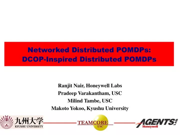
Networked Distributed POMDPs: DCOP-Inspired Distributed POMDPs. Ranjit Nair, Honeywell Labs Pradeep Varakantham, USC Milind Tambe, USC Makoto Yokoo, Kyushu University. Background: DPOMDP. Distributed Partially Observable Markov Decision Problems (DPOMDP): a decision theoretic approach

E N D
Networked Distributed POMDPs: DCOP-Inspired Distributed POMDPs Ranjit Nair, Honeywell Labs Pradeep Varakantham, USC Milind Tambe, USC Makoto Yokoo, Kyushu University
Background: DPOMDP • Distributed Partially Observable Markov Decision Problems (DPOMDP): a decision theoretic approach • Performance linked to optimality of decision making • Explicitly reasons about (+/-ve) rewards and uncertainty. • Current methods use centralized planning and distributed execution • The complexity of finding optimal policy is NEXP-Complete • In many domains,not all agents can interact or affect each other • Most current DPOMDP algorithms do not exploit locality of interaction Distributed sensors Disaster Rescue simulations Battlefield simulations
Background: DCOP x1 x1 di djf(di,dj) 1 2 2 0 Cost = 0 Cost = 7 x2 x2 x3 x4 x3 x4 • Distributed Constraint Optimization Problem (DCOP): • Constraint Graph (V,E) • Vertices are agent’s variables (x1, ..,, x4) each with a domain d1, …, d4 • Edges represent rewards • DCOP algorithms exploit locality of interaction • DCOP algorithms do not reason about uncertainty
Key ideas and contributions • Key ideas: • Exploit locality of interaction to enable scale-up • Hybrid DCOP –DPOMDP approach to collaboratively find joint policy • Distributed offline planning and distributed execution • Key contributions: • ND-POMDP • Distributed POMDP model that captures locality of interaction • Locally Interacting Distributed Joint Equilibrium-based Search for Policies (LID-JESP) • Hill climbing like Distributed Breakout Algorithm (DBA) • Distributed Parallel Algorithm for Finding Locally Optimal Joint Policy • Globally Optimal Algorithm (GOA) • Variable Elimination
Outline • Sensor net domain • Networked Distributed POMDPs (ND-POMDPs) • Locally interacting distributed joint equilibrium-based search for policies (LID-JESP) • Globally optimal algorithm • Experiments • Conclusions and Future Work
Example Domain Ag2 Ag3 Ag1 target1 target2 N W E Sec2 Sec1 S Sec3 Sec4 Sec5 Ag5 Ag4 • Two independent targets • Each changes position based on its stochastic transition function • Sensing agents cannot affect each other or target’s position • False positives and false negatives in observing targets possible • Reward obtained if two agents track a target correctly together • Cost for leaving sensor on
Networked Distributed POMDP • ND-POMDP for set of n agents Ag:<S, A, P, O, Ω, R, b> • World state s ∈ S where S = S1× …× Sn× Su • Each agent i ∈ Ag has local state si∈ Si • E.g. Is sensor on or off? • Su is the part of the state that no agent can affect • E.g. Location of the two targets • b is the initial belief state, a probability distribution over S • b = b1… bn. bu • A = A1× …× An , where Ai is set of actions for agent i • E.g. “Scan East”, “Scan West”, “Turn Off” • No communication during execution • Agents communicate during planning
ND-POMDP • Transition independence: Agent i’s local state cannot be affected by other agents • Pi : Si × Su × Ai × Si → [0,1] • Pu : Su × Su → [0,1] • Ω = Ω1× …× Ωn , where Ωi is set of observations for agent i • E.g. Target present in sector • Observation independence: Agent i’s observations not dependent on others • Oi: Si× Su × Ai × Ωi → [0,1] • Reward function R is decomposable • R(s,a) = ∑lRl (sl1, … slk, su, al1, … alk) • l Ag, and k = |l| • Goal: To find a joint policy π = < π1, …, πn> where πi is the local policy of agent i such that πmaximizes the expected joint reward over finite horizon T
ND-POMDP as a DCOP Ag1 Ag2 Ag3 R12 R1 Ag5 Ag4 • Inter-agent interactions captured by an interaction hypergraph (Ag, E) • Each agent is a node • Set of hyperedges E = {l| l Ag and Rlis a component of R} • Neighborhood of agent i: Set of i’s neighbors • Ni = {j ∈ Ag| j ≠ i, l∈ E,i ∈ l and j ∈ l} • Agents are solving a DCOP where: • Constraint graph is the interaction hypergraph • Variable at each node is the local policy of that agent • Optimize expected joint reward R1: Ag1’s cost for scanning R12: Reward for Ag1 and Ag2 tracking target
ND-POMDP theorems • Theorem 1: For an ND-POMDP, expected reward for a policy is the sum of expected rewards for each of the links for policy • Global value function is decomposable into value functions for each link • Local Neighborhood Utility: V[Ni]: Expected reward obtained from all links involving agent i for executing policy • Theorem 2: Locality of interaction: For policies and ’, if i = ’i and Ni = ’Ni then V[Ni] = V’[Ni] • Given its neighbor’s policies, local neighborhood utility of agent i does not depend on any non-neighbor’s policy
LID-JESP • LID-JESP Algorithm (based on Distributed Breakout Algorithm): • Choose local policy randomly • Communicate local policy to neighbors • Compute local neighborhood utility of current policy wrt to neighbors’ policies • Compute local neighborhood utility of best response policy wrt neighbors (GetValue) • Communicate the gain (4 - 3) to neighbors • If gain is greater than gain of neighbors • Change local policy to best response policy • Communicate changed policy to neighbors • Else • If not reached termination go to step 3 • Theorem 3: Global Utility is strictly increasing with each iteration until local optimum is reached
Termination Detection • Each agent maintains a termination counter • Reset to zero is gain > 0 else increment by 1 • Exchange counter with neighbors • Set counter to min of own counter and neighbors’ counters • Termination detected if counter = d (diameter of graph) • Theorem 4: LID-JESP will terminate within d cycles of reaching local optimum • Theorem 5: If LID-JESP terminates, agents are in a local optimum • From Theorems 3-5, LID-JESP will terminate in a local optimum within d cyles
Computing best response policy • Given neighbors’ fixed policies, each agent is faced with solving a single agent POMDP • State is • Note: state is not fully observable • Transition function: • Observation function: • Reward function: • Best response computed using Bellman backup approach
Global Optimal Algorithm (GOA) • Similar to variable elimination • Relies on a tree structured interaction graph • Cycle cutset algorithm to eliminate cycles • Assumes only binary interactions • Phase 1: Values are propagated upwards from leaves to root • For each policy, sum up values of its children’s optimal responses • Compute value of optimal response to each of the parent’s policies • Communicate these values to parent • Phase 2: Policies are propagated downwards from root to leaves. • Agent chooses policy corresponding to optimal response to parent’s policy • Communicates its policy to child
Experiments Compared to: LID-JESP-no-n/w: ignores interaction graph JESP: Centralized solver (Nair2003) • 3 agent chain • LID-JESP exponentially faster than GOA • 4 agent chain • LID-JESP is faster than JESP and LID-JESP-no-nw • LID-JESP exponentially faster than GOA
Experiments • 5 agent chain • LID-JESP is much faster than JESP and LID-JESP-no-nw • Values: • LID-JESP values are comparable to GOA • Random restarts can be used to find global optimal
Experiments • Reasons for speedup: • C: No. of cycles • G: No. of GetValue calls • W: No. of agents that change their policies in a cycle • LID-JESP converges in fewer cycles (column C) • LID-JESP allows multiple agents to change their policies in a single cycle (column W) • JESP has fewer GetValue calls than LID-JESP • But each such call was slower
Complexity • Complexity of best response: • JESP: O(|S|2. |Ai|. ∏j|Ωj|T) • depends on entire world state • depends on observation histories of all agents • LID-JESP: O(|Su×Si×SNi|2. |Ai|. ∏jNi|Ωj|T) • depends on observation histories of only neighbors • depends only on Su, Si and SNi • Increasing number of agents does not affect complexity • Fixed number of neighbors • Complexity of GOA: • Brute force global optimal: O(∏j|πj|.|S|2.∏j|Ωj|T) • GOA: O(n.|πj|.|Su×Si×Sj|2. |Ai|.|Ωi|T.|Ωj|T) • Increasing number of agents will cause linear increase run time
Conclusions • DCOP algorithms are applied to finding solution to Distributed POMDP • Exploiting “locality of interaction” reduces run time • LID-JESP based on DBA • Agents converge to locally optimal joint policy • GOA based on variable elimination • First distributed parallel algorithms for Distributed POMDPs • Exploiting “locality of interaction” reduces run time • Complexity increases linearly with increased number of agents • Fixed number of neighbors
Future Work • How can communication be incorporated? • Will introducing communication cause agents to lose locality of interaction • Remove assumption of transition independence • May cause all agents to be dependent on each other • Other globally optimal algorithms • Increased parallelism
Global Optimal • Consider only binary constraints. Can be applied to n-ary constraints • Run distributed cycle cutset algorithm in case graph is not a tree • Algorithm: • Convert graph into trees and a cycle cutset C • For each possible joint policy πCof agents in C • Val[πC] = 0 • For each tree of agents • Val[πC] = + DP-Global (tree, πC) • Choose joint policy with highest value
Global Optimal Algorithm (GOA) • Similar to variable elimination • Relies on a tree structured interaction graph • Cycle cutset algorithm to eliminate cycles • Assumes only binary interactions • Phase 1: Values are propagated upwards from leaves to root From the deepest nodes in the tree to the root, do 1. For each of agent i’s policies, πido eval(πi) ←∑ci valueπi ci where valueπi ci is received from child ci. 2. for each parent's policy πj do valueπji ← 0 for each of agent i’s policy πi do set current-eval ← expected-reward(πj , πi) + eval(πi) if valueπji < current-eval then valueπji ← current-eval send valueπji to parent j; • Phase 2: Policies are propagated downwards from root to leaves.